Home Discussion Topics Dictionary Almanac

Signup Login

Curvilinear coordinates

Overview

Curvilinear coordinates are a coordinate system

Coordinate system

In mathematics and its applications, a coordinate system is a system for assigning an n-tuple of numbers or scalars to each point in an n-dimensional space. This concept is part of the theory of manifolds. "Scalars" in many cases means real numbers, but, depending on context, can mean complex...

for the Euclidean space

Euclidean space

In mathematics, Euclidean space is the Euclidean plane and three-dimensional space of Euclidean geometry, as well as the generalizations of these notions higher dimensions...

Discussion

Ask a question about 'Curvilinear coordinates'

Start a new discussion about 'Curvilinear coordinates'

Answer questions from other users

Full Discussion Forum

Encyclopedia

Curvilinear coordinates are a coordinate system

Coordinate system

for the Euclidean space

Euclidean space

In mathematics, Euclidean space is the Euclidean plane and three-dimensional space of Euclidean geometry, as well as the generalizations of these notions higher dimensions...

based on some transformation that converts the standard Cartesian coordinate system to a coordinate system with the same number of coordinates in which the coordinate lines are curved. In the two-dimensional case, instead of Cartesian coordinates x and y, e.g., p and q are used: the level curves of p and q in the xy-plane. Required is that the transformation is locally invertible (a one-to-one map) at each point. This means that one can convert a point given in one coordinate system to its curvilinear coordinates and back.

Depending on the application, a curvilinear coordinate system may be simpler to use than the Cartesian coordinate system.
For instance, a physical problem with spherical symmetry defined in R³ (e.g., motion in the field of a point mass/charge),
is usually easier to solve in spherical polar coordinates than in Cartesian coordinates. Also boundary conditions may enforce symmetry. One would describe the motion of a particle in a rectangular box in Cartesian coordinates, whereas one would prefer spherical coordinates for a particle in a sphere.

Many of the concepts in vector calculus

Vector calculus

Vector calculus is a branch of mathematics concerned with differentiation and integration of vector fields. The term "vector calculus" is sometimes used as a synonym for the broader subject of multivariable calculus, which includes vector calculus as well as partial differentiation and multiple...

, which are given in Cartesian or spherical polar coordinates, can be formulated in arbitrary curvilinear coordinates.
This gives a certain economy of thought, as it is possible to derive general expressions—valid for any curvilinear coordinate system—for concepts as gradient, divergence, curl, and the Laplacian.
Well-known examples of curvilinear systems are polar coordinates for R²,
and cylinder

Cylindrical coordinate system

A cylindrical coordinate system is a three-dimensional coordinate system, where each point is specified by the two polar coordinates of its perpendicular projection onto some fixed plane, and by its distance from that plane....

and spherical polar coordinates for R³.

The name curvilinear coordinates, coined by the French mathematician Lamé

Gabriel Lamé

Père de Gabriel Léon Jean Baptiste Lamé was a French mathematician.-Biography:Lamé was born in Tours, in today's département of Indre-et-Loire....

, derives from the fact that the coordinate surface

Coordinate surface

The coordinate surfaces of a three dimensional coordinate system are the surfaces on which a particular coordinate of the system is constant, while the coordinate lines are the curves along which two of the coordinates of the system are constant...

s of the curvilinear systems are curved. While a Cartesian coordinate surface is a plane, e.g., z = 0 defines the x-y plane, the coordinate surface r = 1 in spherical polar coordinates is the surface of a unit sphere in R³—which obviously is curved.

General curvilinear coordinates

In Cartesian coordinates, the position of a point P(x,y,z) is determined by the intersection of three mutually perpendicular planes, x = const, y = const, z = const. The coordinates x, y and z are related to three new quantities q₁,q₂, and q₃ by the equations:

x = x(q₁,q₂,q₃) direct transformation

y = y(q₁,q₂,q₃) (curvilinear to Cartesian coordinates)

z = z(q₁,q₂,q₃)

The above equation system can be solved for the arguments q₁, q₂, and q₃ with solutions in the form:

q₁ = q₁(x, y, z) inverse transformation

q₂ = q₂(x, y, z) (Cartesian to curvilinear coordinates)

q₃ = q₃(x, y, z)

The transformation functions are such that there's a one-to-one relationship between points in the "old" and "new" coordinates, that is, those functions are bijection

Bijection

In mathematics, a bijection, or a bijective function is a function f from a set X to a set Y with the property that, for every y in Y, there is exactly one x in X such that f = y and no unmapped element remains in both X and Y.Alternatively, f is bijective if it is a one-to-one correspondence...

s, and fulfil the following requirements within their domain

Domain

-General:* some kind of territory , such as a demesne or a realm* a field of study* public domain, a body of works and knowledge without proprietary interest...

1) They are smooth function

Smooth function

In mathematical analysis, a differentiability class is a classification of functions according to the properties of their derivatives. Higher order differentiability classes correspond to the existence of more derivatives. Functions that have derivatives of all orders are called smooth.Most of...

2) The Jacobian

Jacobian

In vector calculus, the Jacobian matrix is the matrix of all first-order partial derivatives of a vector-valued function. Suppose F : Rⁿ → R^m is a function from Euclidean n-space to Euclidean m-space...

determinant

is not zero; that is, the transformation is invertible according to the inverse function theorem

Inverse function theorem

In mathematics, specifically differential calculus, the inverse function theorem gives sufficient conditions for a function to be invertible in a neighborhood of a point in its domain...

. The condition that the Jacobian determinant is not zero reflects the fact that three surfaces from different families intersect in one and only one point and thus determine the position of this point in a unique way.

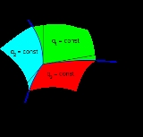
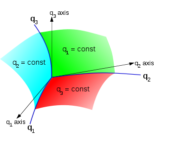
A given point may be described by specifying either x, y, z or q₁, q₂, q₃ while each of the inverse equations describes a surface in the new coordinates and the intersection of three such surfaces locates the point in the three-dimensional space (Fig. 1). The surfaces q₁ = const, q₂ = const, q₃ = const are called the coordinate surfaces; the space curves formed by their intersection in pairs are called the coordinate lines. The coordinate axes are determined by the tangents to the coordinate lines at the intersection of three surfaces. They are not in general fixed directions in space, as is true for simple Cartesian coordinates. The quantities (q₁, q₂, q₃ ) are the curvilinear coordinates of a point P(q₁, q₂, q₃ ).

In general, (q₁, q₂ ... q_n ) are curvilinear coordinates in n-dimensional space.

Curvilinear Coordinates from a Mathematical Perspective

From a more general and abstract perspective, a curvilinear coordinate system is simply a coordinate patch

Atlas (topology)

In mathematics, particularly topology, an atlas describes how a manifold is equipped with a differential structure. Each piece is given by a chart ....

on the differential manifold Eⁿ (n-dimensional Euclidian space) that is diffeomorphic to the Cartesian coordinate patch on the manifold. Note that two diffeomorphic coordinate patches on a differential manifold need not overlap differentiably. With this simple definition of a curvilinear coordinate system, all the results that follow below are simply applications of standard theorems in differential topology

Differential topology

In mathematics, differential topology is the field dealing with differentiable functions on differentiable manifolds. It is closely related to differential geometry and together they make up the geometric theory of differentiable manifolds.- Description :...

Example: Spherical coordinates

Spherical coordinates are one of the most used curvilinear coordinate systems in such fields as Earth sciences, cartography, and physics (quantum physics, relativity, etc.). The curvilinear coordinates (q₁, q₂, q₃) in this system are, respectively, r (radial distance or polar radius, r ≥ 0), θ (zenith or latitude, 0 ≤ θ ≤ 180°), and φ (azimuth or longitude, 0 ≤ φ ≤ 360°).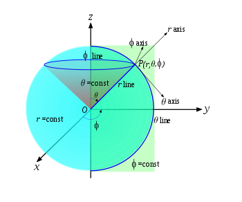
The direct relationship between Cartesian and spherical coordinates is given by:
Solving the above equation system for r, θ, and φ gives the inverse relations between spherical and Cartesian coordinates:

The respective spherical coordinate surfaces are derived in terms of Cartesian coordinates by fixing the spherical coordinates in the above inverse transformations to a constant value. Thus (Fig.2), r = const are concentric spherical surfaces centered at the origin, O, of the Cartesian coordinates, θ = const are circular conical surfaces with apex in O and axis the Oz axis, φ = const are half-planes bounded by the Oz axis and perpendicular to the xOy Cartesian coordinate plane. Each spherical coordinate line is formed at the pairwise intersection of the surfaces, corresponding to the other two coordinates: r lines (radial distance) are beams Or at the intersection of the cones θ = const and the half-planes φ = const; θ lines (meridians) are semicircles formed by the intersection of the spheres r = const and the half-planes φ = const ; and φ lines (parallels) are circles in planes parallel to xOy at the intersection of the spheres r = const and the cones θ = const. The location of a point P(r,θ,φ) is determined by the point of intersection of the three coordinate surfaces, or, alternatively, by the point of intersection of the three coordinate lines. The θ and φ axes in P(r,θ,φ) are the mutually perpendicular (orthogonal) tangents to the meridian and parallel of this point, while the r axis is directed along the radial distance and is orthogonal to both θ and φ axes.

The surfaces described by the inverse transformations are smooth functions within their defined domains. The Jacobian (functional determinant) of the inverse transformations is:

Curvilinear local basis

Coordinates are used to define location or distribution of physical quantities which are scalar

Scalar (mathematics)

In linear algebra, real numbers are called scalars and relate to vectors in a vector space through the operation of scalar multiplication, in which a vector can be multiplied by a number to produce another vector....

s, vectors, or tensor

Tensor

Tensors are geometrical entities introduced into mathematics and physics to extend the notion of scalars, vectors, and matrices. Many physical quantities are naturally regarded, not as vectors themselves, but as correspondences between one set of vectors and another...

s. Scalars are expressed as points and their location is defined by specifying their coordinates with the use of coordinate lines or coordinate surfaces. Vectors are objects that possess two characteristics: magnitude and direction.

The concept of a basis

To define a vector in terms of coordinates, an additional coordinate-associated structure, called basis

Basis (linear algebra)

In linear algebra, a basis is a set of vectors that, in a linear combination, can represent every vector in a given vector space or free module, and such that no element of the set can be represented as a linear combination of the others...

, is needed. A basis in three-dimensional space is a set of three linearly independent

Linear independence

In linear algebra, a family of vectors is linearly independent if none of them can be written as a linear combination of finitely many other vectors in the collection. A family of vectors which is not linearly independent is called linearly dependent...

vector

Coordinate vector

In linear algebra, a coordinate vector is an explicit representation of a vector in an abstract vector space as an ordered list of numbers or, equivalently, as an element of the coordinate space Fⁿ....

s {e₁, e₂, e₃}, called basis vectors. Each basis vector is associated with a coordinate in the respective dimension. Any vector can be represented as a sum of vectors A_ne_n formed by multiplication of a basis vector by a scalar coefficient, called component. Each vector, then, has exactly one component in each dimension and can be represented by the vector sum: A = A₁e₁ + A₂e₂ + A₃e₃, where A_n and e_n are the respective components and basis vectors. A requirement for the coordinate system and its basis is that A₁e₁ + A₂e₂ + A₃e₃ ≠ 0 when at least one of the A_n ≠ 0. This condition is called linear independence

Linear independence

. Linear independence implies that there cannot exist bases with basis vectors of zero magnitude because the latter will give zero-magnitude vectors when multiplied by any component. Non-coplanar vectors are linearly independent, and any triple of non-coplanar vectors can serve as a basis in three dimensions.

Basis vectors in curvilinear coordinates

For the general curvilinear coordinates, basis vectors and components vary from point to point. If vector A whose origin is in point P (q₁, q₂, q₃ ) is moved to point P' (q'₁, q'₂, q'₃ ) in such a way that its direction and orientation are preserved, then the moved vector will be expressed by new components A'_n and basis vectors e^'n. Therefore, the vector sum that describes vector A in the new location is composed of different vectors, although the sum itself remains the same. A coordinate basis whose basis vectors change their direction and/or magnitude from point to point is called local basis. All bases associated with curvilinear coordinates are necessarily local. Global bases, that is, bases composed of basis vectors that are the same in all points can be associated only with linear coordinates. A more exact, though seldom used, expression for such vector sums with local basis vectors is , where the dependence of both components and basis vector on location is made explicit (n is the number of dimensions). Local bases are composed of vectors with arbitrary order, magnitude, and direction and magnitude/direction vary in different points in space.

Choosing an appropriate basis

Basis vectors are usually associated with a coordinate system by two methods:

they can be built along the coordinate axes (colinear with axes) or
they can be built to be perpendicular (normal) to the coordinate surfaces.

In the first case (axis-collinear), basis vectors transform like covariant vectors while in the second case (normal to coordinate surfaces), basis vectors transform like contravariant vectors. Those two types of basis vectors are distinguished by the position of their indices: covariant vectors are designated with lower indices while contravariant vectors are designated with upper indices. Thus, depending on the method by which they are built, for a general curvilinear coordinate system there are two sets of basis vectors for every point: {e₁, e₂, e₃} is the covariant basis, and {e¹, e², e³} is the contravariant basis.

Covariant and contravariant bases

A key property of the vector and tensor representation in terms of indexed components and basis vectors is invariance in the sense that vector components which transform in a covariant manner (or contravariant manner) are paired with basis vectors that transform in a contravariant manner (or covariant manner), and these operations are inverse to one another according to the transformation rules. This means that in terms, in which an index occurs two times, one of the indices in the pair must be upper and the other index must be lower. Thus in the above vector sums, basis vectors with lower indices are multiplied by components with upper indices or vice versa, so that a given vector can be represented in two ways: A = A¹e₁ + A²e₂ + A³e₃ = A₁e¹ + A₂e² + A₃e³. Upon coordinate change, a vector transforms in the same way as its components. Therefore, a vector is covariant or contravariant if, respectively, its components are covariant or contravariant. From the above vector sums, it can be seen that contravariant vectors are represented with covariant basis vectors, and covariant vectors are represented with contravariant basis vectors. This is reflected in the Einstein summation convention

Einstein notation

In mathematics, especially in applications of linear algebra to physics, the Einstein notation or Einstein summation convention is a notational convention useful when dealing with coordinate formulas...

according to which in the vector sums and the basis vectors and the summation symbols are omitted, leaving only Aⁱ and A_i which represent, respectively, a contravariant and a covariant vector.

Covariant basis

As stated above, contravariant vectors are vectors with contravariant components whose location is determined using covariant basis vectors that are built along the coordinate axes. In analogy to the other coordinate elements, transformation of the covariant basis of general curvilinear coordinates is described starting from the Cartesian coordinate system
Cartesian coordinate system
A Cartesian coordinate system specifies each point uniquely in a plane by a pair of numerical coordinates, which are the signed distances from the point to two fixed perpendicular directed lines, measured in the same unit of length....

whose basis is called standard basis
Standard basis
In mathematics, the standard basis for a Euclidean space consists of one unit vector pointing in the direction of each axis of the Cartesian coordinate system...

. The standard basis is a global basis that is composed of 3 mutually orthogonal vectors {i, j, k} of unit length, that is, the magnitude of each basis vector equals 1. Regardless of the method of building the basis (axis-collinear or normal to coordinate surfaces), in the Cartesian system the result is a single set of basis vectors, namely, the standard basis. To avoid misunderstanding, in this section the standard basis will be thought of as built along the coordinate axes.

Constructing a covariant basis in one dimension

Consider the one-dimensional curve shown in Fig. 3. At point P, taken as an origin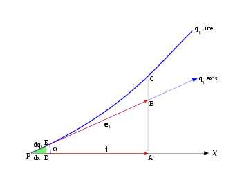
Origin (mathematics)
In mathematics, the origin of a Euclidean space is a special point, usually denoted by the letter O, used as a fixed point of reference for the geometry of the surrounding space. In a Cartesian coordinate system, the origin is the point where the axes of the system intersect...

, x is one of the Cartesian coordinates, and q₁ is one of the curvilinear coordinates (Fig. 3). The local basis vector is e₁ and it is built on the q₁ axis which is a tangent to q₁ coordinate line at the point P. The axis q₁ and thus the vector e₁ form an angle α with the Cartesian x axis and the Cartesian basis vector i.

It can be seen from triangle PAB that where |e₁| is the magnitude of the basis vector e₁ (the scalar intercept PB) and |i| is the magnitude of the Cartesian basis vector i which is also the projection of e₁ on the x axis (the scalar intercept PA). It follows, then, that and .

However, this method for basis vector transformations using directional cosines is inapplicable to curvilinear coordinates for the following reason. With increasing the distance from P, the angle between the curved line q₁ and Cartesian axis x increasingly deviates from α. At the distance PB the true angle is that which the tangent at point C forms with the x axis and the latter angle is clearly different from α. The angles that the q₁ line and q₁ axis form with the x axis become closer in value the closer one moves towards point P and become exactly equal at P. Let point E is located very close to P, so close that the distance PE is infinitesimally small. Then PE measured on the q₁ axis almost coincides with PE measured on the q₁ line. At the same time, the ratio (PD being the projection of PE on the x axis) becomes almost exactly equal to cos α.

Let the infinitesimally small intercepts PD and PE be labelled, respectively, as dx and dq₁. Then
and .

Thus, the directional cosines can be substituted in transformations with the more exact ratios between infinitesimally small coordinate intercepts.

If and are smooth (continuously differentiable) functions and, therefore, the transformation ratios can be written as and ,

that is, those ratios are partial derivative

Partial derivative

In mathematics, a partial derivative of a function of several variables is its derivative with respect to one of those variables with the others held constant...

s of coordinates belonging to one system with respect to coordinates belonging to the other system.

From the foregoing discussion, it follows that the component (projection) of e₁ on the x axis is
.

Therefore the projection of the normalized local basis vector (|e₁| = 1) can be made a vector directed along the x axis by multiplying it with the standard basis vector i.

Constructing a covariant basis in three dimensions

Doing the same for the coordinates in the other 2 dimensions, e₁ can be expressed as: . Similar equations hold for e₂ and e₃ so that the standard basis {i, j, k} is transformed to local (ordered and normalised) basis {e₁, e₂, e₃} by the following system of equations:
Vectors e₁, e₂, and e₃ at the right hand side of the above equation system are unit vectors (magnitude = 1) directed along the 3 axes of the curvilinear coordinate system. However, basis vectors in general curvilinear system are not required to be of unit length: they can be of arbitrary magnitude and direction. It can easily be shown that the condition |e₁| = |e₂| = |e₃| = 1 is a result of the above transformation, and not an a priori requirement imposed on the curvilinear basis. Let the local basis {e₁, e₂, e₃} not be normalised, in effect, leaving the basis vectors with arbitrary magnitudes. Then, instead of e₁, e₂, and e₃ in the right hand side, there will be , , and which are again unit vectors directed along the curvilinear coordinate axes.

By analogous reasoning, but this time projecting the standard basis on the curvilinear axes ( |i| = |j| = |k| = 1 according to the definition of standard basis
Standard basis
In mathematics, the standard basis for a Euclidean space consists of one unit vector pointing in the direction of each axis of the Cartesian coordinate system...

), one can obtain the inverse transformation from local basis to standard basis:

Transformation between curvilinear and Cartesian coordinates

The above systems of linear equations can be written in matrix form as and where x_i (i = 1,2,3) are the Cartesian coordinates x, y, z and i_i are the standard basis vectors i, j, k. The system matrices (that is, matrices composed of the coefficients in front of the unknowns) are, respectively, and . At the same time, those two matrices are the Jacobian matrices

Jacobian

J_ik and J⁻¹_ik of the transformations of basis vectors from curvilinear to Cartesian coordinates and vice versa. In the second equation system (the inverse transformation), the unknowns are the curvilinear basis vectors which are subject to the condition that in each point of the curvilinear coordinate system there must exist one and only one set of basis vectors. This condition is satisfied iff (if and only if) the equation system has a single solution.

From linear algebra

Linear algebra

Linear algebra is a branch of mathematics concerned with the study of vectors, vector spaces , linear maps , and systems of linear equations. Vector spaces are a central theme in modern mathematics; thus, linear algebra is widely used in both abstract algebra and functional analysis...

, it is known that a linear equation system has a single solution only if the determinant of its system matrix is non-zero. For the second equation system, the determinant of the system matrix is which shows the rationale behind the above requirement concerning the inverse Jacobian determinant.

Another, very important, feature of the above transformations is the nature of the derivatives: in front of the Cartesian basis vectors stand derivatives of Cartesian coordinates while in front of the curvilinear basis vectors stand derivatives of curvililear coordinates. In general, the following definition holds:

This definition is so general that it applies to covariance

Covariance and contravariance

In multilinear algebra and tensor analysis, covariance and contravariance describe how the quantitative description of certain geometrical or physical entities changes when passing from one coordinate system to another. The coordinates of a geometrical vector can be measured with respect to a...

in the very abstract sense, and includes not only basis vectors, but also all vectors, components, tensors, pseudovectors, and pseudotensors (in the last two there is an additional sign flip). It also serves to define tensors in one of their most usual treatments

Intermediate treatment of tensors

In mathematics and physics, a tensor is an idealized geometric or physical quantity whose numerical description, relative to a particular frame of reference, consists of a multiple indexed array of numbers. A vector, for example, is a tensor with a single index; thus, tensors can be regarded as...

Lamé coefficients

The partial derivative coefficients through which vector transformation is achieved are called also scale factors or Lamé coefficients (named after Gabriel Lamé

Gabriel Lamé

Père de Gabriel Léon Jean Baptiste Lamé was a French mathematician.-Biography:Lamé was born in Tours, in today's département of Indre-et-Loire....

): . However, the h_ik designation is very rarely used, being largely replaced with √g_ik, the components of the metric tensor

Metric tensor

In the mathematical field of differential geometry, a metric tensor is a type of function defined on a manifold which takes as input a pair of tangent vectors v and w and produces a real number g in a way that generalizes many of the familiar properties of the dot product of vectors in Euclidean...

Vector and tensor algebra in three-dimensional curvilinear coordinates

Vectors in curvilinear coordinatess

Let be an arbitrary basis for three-dimensional Euclidean space. In general, the basis vectors are neither unit vectors nor mutually orthogonal. However, they are required to be linearly independent. Then a vector can be expressed as
The components are the contravariant components of the vector .

The reciprocal basis is defined by the relation
where is the Kronecker delta

Kronecker delta

In mathematics, the Kronecker delta or Kronecker's delta, named after Leopold Kronecker , is a function of two variables, usually integers, which is 1 if they are equal, and 0 otherwise...

.

The vector can also be expressed in terms of the reciprocal basis:
The components are the covariant components of the vector .

Relations between components and basis vectors

From these definitions we can see that
Also,

Second-order tensors in curvilinear coordinates

A second-order tensor can be expressed as
The components are called the contravariant components, the mixed right-covariant components, the mixed left-covariant components, and the covariant components of the second-order tensor.

Action of a second-order tensor on a vector

The action can be expressed in curvilinear coordinates as

Inner product of two second-order tensors

The inner product of two second-order tensors can be expressed in curvilinear coordinates as
Alternatively,

Determinant of a second-order tensor

If is a second-order tensor, then the determinant is defined by the relation
where are arbitrary vectors and

Vector and tensor calculus in three-dimensional curvilinear coordinates

Let the position of a point in space be characterized by three coordinate variables . The coordinate curve represents a surface on which are constant. Let be the position vector

Position vector

A position, location, or radius vector is a vector which represents the position of an object in space in relation to an arbitrary reference point. The concept applies to two- or three-dimensional space...

of the point relative to some origin. Then, assuming that such a mapping and its inverse exist and are continuous, we can write
The fields are called the curvilinear coordinate functions of the curvilinear coordinate system .

The coordinate curves are defined by the one-parameter family of functions given by
with fixed.

Tangent vector to coordinate curves

The tangent vector to the curve at the point (or to the coordinate curve at the point ) is

Gradient of a scalar field

Let be a scalar field in space. Then
The gradient of the field is defined by
where is an arbitrary constant vector. If we define the components of vector such that
then

If we set , then since , we have
which provides a means of extracting the contravariant component of a vector .

If is the covariant (or natural) basis at a point, and if is the contravariant (or reciprocal) basis at that point, then
A brief rationale for this choice of basis is given in the next section.

Gradient of a vector field

A similar process can be used to arrive at the gradient of a vector field . The gradient is given by
If we consider the gradient of the position vector field , then we can show that
The vector field is tangent to the coordinate curve and forms a natural basis at each point on the curve. This basis, as discussed at the beginning of this article, is also called the covariant curvilinear basis. We can also define a reciprocal basis, or contravariant curvilinear basis, . All the algebraic relations between the basis vectors, as discussed in the section on tensor algebra, apply for the natural basis and its reciprocal at each point .

Since is arbitrary, we can write

Note that the contravariant basis vector is perpendicular to the surface of constant and is given by

Christoffel symbols of the second kind

The Christoffel symbols of the second kind is defined as
This implies that
Other relations that follow are

Another particularly useful relation, which shows that the Christoffel symbol depends only on the metric tensor and its derivatives, is

Explicit expression for the gradient of a vector field

The following expressions for the gradient of a vector field in curvilinear coordinates are quite useful.

Representing a physical vector field

The vector field can be represented as
where are the covariant components of the field, are the physical components, and
is the normalized contravariant basis vector.

Divergence of a vector field

The divergence

Divergence

In vector calculus, the divergence is an operator that measures the magnitude of a vector field's source or sink at a given point; the divergence of a vector field is a scalar. For example, consider air as it is heated or cooled. The relevant vector field for this example is the velocity of the...

of a vector field is defined as
In terms of components with respect to a curvilinear basis

Alternative expression for the divergence of a vector field

An alternative equation for the divergence of a vector field is frequently used. To derive this relation recall that
Now,
Noting that, due to the symmetry of ,
we have
Recall that if is the matrix whose components are , then the inverse of the matrix is . The inverse of the matrix is given by
where are the cofactor matrices of the components . From matrix algebra we have
Hence,
Plugging this relation into the expression for the divergence gives
A little manipulation leads to the more compact form

Laplacian of a scalar field

The Laplacian of a scalar field is defined as
Using the alternative expression for the divergence of a vector field gives us
Now
Therefore,

Gradient of a second-order tensor field

The gradient of a second order tensor field can similarly be expressed as

Explicit expressions for the gradient

If we consider the expression for the tensor in terms of a contravariant basis, then
We may also write

Representing a physical second-order tensor field

The physical components of a second-order tensor field can be obtained by using a normalized contravariant basis, i.e.,
where the hatted basis vectors have been normalized. This implies that

Divergence of a second-order tensor field

The divergence

Divergence

of a second-order tensor field is defined using
where is an arbitrary constant vector.

In curvilinear coordinates,

Relations between curvilinear and Cartesian basis vectors

Let be the usual Cartesian basis vectors for the Euclidean space of interest and let
where is a second-order transformation tensor that maps to . Then,
From this relation we can show that
Let be the Jacobian of the transformation. Then, from the definition of the determinant,
Since
we have
A number of interesting results can be derived using the above relations.

First, consider
Then
Similarly, we can show that
Therefore, using the fact that ,

Another interesting relation is derived below. Recall that
where is a, yet undetermined, constant. Then
This observation leads to the relations
In index notation,
where is the usual permutation symbol.

We have not identified an explicit expression for the transformation tensor because an alternative form of the mapping between curvilinear and Cartesian bases is more useful. Assuming a sufficient degree of smoothness in the mapping (and a bit of abuse of notation), we have
Similarly,
From these results we have
and

Vector products

The cross product

Cross product

In mathematics, the cross product is a binary operation on two vectors in a three-dimensional Euclidean space that results in another vector which is perpendicular to the plane containing the two input vectors. The algebra defined by the cross product is neither commutative nor associative. It...

of two vectors is given by
where is the permutation symbol and is a Cartesian basis vector. Therefore,
and
Hence,
Returning back to the vector product and using the relations
gives us

The alternating tensor

In an orthonormal right-handed basis, the third-order alternating tensor is defined as
In a general curvilinear basis the same tensor may be expressed as
It can be shown that
Now,
Hence,
Similarly, we can show that

Example: Cylindrical polar coordinates

For cylindrical coordinates we have
and
where

Then the covariant and contravariant basis vectors are
where are the unit vectors in the directions.

Note that the components of the metric tensor are such that
which shows that the basis is orthogonal.

The non-zero components of the Christoffel symbol of the second kind are

Representing a physical vector field

The normalized contravariant basis vectors in cylindrical polar coordinates are
and the physical components of a vector are

Gradient of a scalar field

The gradient of a scalar field, , in cylindrical coordinates can now be computed from the general expression in curvilinear coordinates and has the form

Gradient of a vector field

Similarly, the gradient of a vector field, , in cylindrical coordinates can be shown to be

Divergence of a vector field

Using the equation for the divergence of a vector field in curvilinear coordinates, the divergence in cylindrical coordinates can be shown to be

Representing a physical second-order tensor field

The physical components of a second-order tensor field are those obtained when the tensor is expressed in terms of a normalized contravariant basis. In cylindrical polar coordinates these components are

Gradient of a second-order tensor field

Using the above definitions we can show that the gradient of a second-order tensor field in cylindrical polar coordinates can be expressed as

Divergence of a second-order tensor field

The divergence of a second-order tensor field in cylindrical polar coordinates can be obtained from the expression for the gradient by collecting terms where the scalar product of the two outer vectors in the dyadic products is nonzero. Therefore,

Orthogonal curvilinear coordinates

Assume, for the purposes of this section, that the curvilinear coordinate system is orthogonal, i.e.,
where are covariant basis vectors, are contravariant basis vectors. Also, let be a background, fixed, Cartesian basis.

Metric tensor in orthogonal curvilinear coordinates

Let be the position vector

Position vector

of the point with respect to the origin of the coordinate system. The notation can be simplified by noting that . At each point we can construct a small line element . The square of the length of the line element is the scalar product and is called the metric

Metric (mathematics)

In mathematics, a metric or distance function is a function which defines a distance between elements of a set. A set with a metric is called a metric space. A metric induces a topology on a set but not all topologies can be generated by a metric...

of the space

Space

Space is the boundless, three-dimensional extent in which objects and events occur and have relative position and direction. Physical space is often conceived in three linear dimensions, although modern physicists usually consider it, with time, to be part of the boundless four-dimensional...

. Recall that the space of interest is assumed to be Euclidean

Euclidean space

In mathematics, Euclidean space is the Euclidean plane and three-dimensional space of Euclidean geometry, as well as the generalizations of these notions higher dimensions...

when we talk of curvilinear coordinates. Let us express the position vector in terms of the background, fixed, Cartesian basis, i.e.,

Using the chain rule

Chain rule

In calculus, the chain rule is a formula for the derivative of the composite of two functions.In intuitive terms, if a variable, y, depends on a second variable, u, which in turn depends on a third variable, x, then the rate of change of y with respect to x can be computed as the rate of change of...

, we can then express in terms of three-dimensional orthogonal curvilinear coordinates as
Therefore the metric is given by

The symmetric quantity
is called the fundamental (or metric) tensor

Metric tensor

of the Euclidean space

Euclidean space

In mathematics, Euclidean space is the Euclidean plane and three-dimensional space of Euclidean geometry, as well as the generalizations of these notions higher dimensions...

in curvilinear coordinates.

Note also that
where are the Lamé coefficients.

If we define the scale factors, , using
we get a relation between the fundamental tensor and the Lamé coefficients.

Example: Polar coordinates

If we consider polar coordinates for R², note that
(r, θ) are the curvilinear coordinates, and the Jacobian determinant of the transformation (r,θ) → (r cos θ, r sin θ) is r.

The orthogonal basis vectors are g_r = (cos θ, sin θ), g_θ = (−r sin θ, r cos θ). The normalized basis vectors are e_r = (cos θ, sin θ), e_θ = (−sin θ, cos θ) and the scale factors are h_r = 1 and h_θ= r. The fundamental tensor is g₁₁ =1, g₂₂ =r², g₁₂ = g₂₁ =0.

Line and surface integrals

If we wish to use curvilinear coordinates for vector calculus

Vector calculus

calculations, adjustments need to be made in the calculation of line, surface and volume integrals. For simplicity, we again restrict the discussion to three dimensions and orthogonal curvilinear coordinates. However, the same arguments apply for -dimensional problems though there are some additional terms in the expressions when the coordinate system is not orthogonal.

Line integrals

Normally in the calculation of line integral

Line integral

In mathematics, a line integral is an integral where the function to be integrated is evaluated along a curve. Various different line integrals are in use...

s we are interested in calculating
where x(t) parametrizes C in Cartesian coordinates.
In curvilinear coordinates, the term
by the chain rule

Chain rule

. And from the definition of the Lamé coefficients,
and thus
Now, since when , we have
and we can proceed normally.

Surface integrals

Likewise, if we are interested in a surface integral

Surface integral

In mathematics, a surface integral is a definite integral taken over a surface ; it can be thought of as the double integral analog of the line integral...

, the relevant calculation, with the parameterization of the surface in Cartesian coordinates is:
Again, in curvilinear coordinates, we have
and we make use of the definition of curvilinear coordinates again to yield

Therefore,
where is the permutation symbol.

In determinant form, the cross product in terms of curvilinear coordinates will be:

Grad, curl, div, Laplacian

In orthogonal

Orthogonality

In mathematics, two vectors are orthogonal if they are perpendicular, i.e., they form a right angle. The word comes from the Greek , meaning "straight", and , meaning "angle".- Definitions :...

curvilinear coordinates of dimensions, where
one can express the gradient

Gradient

In vector calculus, the gradient of a scalar field is a vector field which points in the direction of the greatest rate of increase of the scalar field, and whose magnitude is the greatest rate of change....

of a scalar

Scalar (mathematics)

or vector field

Vector field

In mathematics a vector field is a construction in vector calculus which associates a vector to every point in a subset of Euclidean space.Vector fields are often used in physics to model, for example, the speed and direction of a moving fluid throughout space, or the strength and direction of...

as
For an orthogonal basis
The divergence

Divergence

of a vector field can then be written as
Also,
Therefore,
We can get an expression for the Laplacian in a similar manner by noting that
Then we have
The expressions for the gradient, divergence, and Laplacian can be directly extended to -dimensions.

The curl of a vector field

Vector field

is given by
where is the product of all
and is the Levi-Civita symbol

Levi-Civita symbol

The Levi-Civita symbol, also called the permutation symbol, antisymmetric symbol, or alternating symbol, is a mathematical symbol used in particular in tensor calculus. It is named after the Italian mathematician and physicist Tullio Levi-Civita.-Definition:In three dimensions, the Levi-Civita...

Fictitious forces in general curvilinear coordinates

An inertial coordinate system is defined as a system of space and time coordinates x₁,x₂,x₃,t in terms of which the equations of motion of a particle free of external forces are simply d²x_j/dt² = 0. In this context, a coordinate system can fail to be “inertial” either due to non-straight time axis or non-straight space axes (or both). In other words, the basis vectors of the coordinates may vary in time at fixed positions, or they may vary with position at fixed times, or both. When equations of motion are expressed in terms of any non-inertial coordinate system (in this sense), extra terms appear, called Christoffel symbols. Strictly speaking, these terms represent components of the absolute acceleration (in classical mechanics), but we may also choose to continue to regard d²x_j/dt² as the acceleration (as if the coordinates were inertial) and treat the extra terms as if they were forces, in which case they are called fictitious forces. The component of any such fictitious force normal to the path of the particle and in the plane of the path’s curvature is then called centrifugal force

Centrifugal force

In classical mechanics, centrifugal force is an outward force associated with curved motion, that is, rotation about some center...

.

This more general context makes clear the correspondence between the concepts of centrifugal force in rotating coordinate system

Rotating reference frame

A rotating frame of reference is a special case of a non-inertial reference frame that is rotating relative to an inertial reference frame. An everyday example of a rotating reference frame is the surface of the Earth. A rotating frame of reference is a special case of a non-inertial reference...

s and in stationary curvilinear coordinate systems. (Both of these concepts appear frequently in the literature.) For a simple example, consider a particle of mass m moving in a circle of radius r with angular speed w relative to a system of polar coordinates rotating with angular speed W. The radial equation of motion is mr” = F_r + mr(w+W)². Thus the centrifugal force is mr times the square of the absolute rotational speed A = w + W of the particle. If we choose a coordinate system rotating at the speed of the particle, then W = A and w = 0, in which case the centrifugal force is mrA², whereas if we choose a stationary coordinate system we have W = 0 and w = A, in which case the centrifugal force is again mrA². The reason for this equality of results is that in both cases the basis vectors at the particle’s location are changing in time in exactly the same way. Hence these are really just two different ways of describing exactly the same thing, one description being in terms of rotating coordinates and the other being in terms of stationary curvilinear coordinates, both of which are non-inertial according to the more abstract meaning of that term.

When describing general motion, the actual forces acting on a particle are often referred to the instantaneous osculating circle tangent to the path of motion, and this circle in the general case is not centered at a fixed location, and so the decomposition into centrifugal and Coriolis components is constantly changing. This is true regardless of whether the motion is described in terms of stationary or rotating coordinates.

Curvilinear coordinates

General curvilinear coordinates

Curvilinear Coordinates from a Mathematical Perspective

Example: Spherical coordinates

Curvilinear local basis

The concept of a basis

Basis vectors in curvilinear coordinates

Choosing an appropriate basis

Covariant and contravariant bases

Covariant basis

Constructing a covariant basis in one dimension

Constructing a covariant basis in three dimensions

Transformation between curvilinear and Cartesian coordinates

Lamé coefficients

Vector and tensor algebra in three-dimensional curvilinear coordinates

Vectors in curvilinear coordinatess

Relations between components and basis vectors

Second-order tensors in curvilinear coordinates

Action of a second-order tensor on a vector

Inner product of two second-order tensors

Determinant of a second-order tensor

Vector and tensor calculus in three-dimensional curvilinear coordinates

Tangent vector to coordinate curves

Gradient of a scalar field

Gradient of a vector field

Christoffel symbols of the second kind

Explicit expression for the gradient of a vector field

Representing a physical vector field

Divergence of a vector field

Alternative expression for the divergence of a vector field

Laplacian of a scalar field

Gradient of a second-order tensor field

Explicit expressions for the gradient

Representing a physical second-order tensor field

Divergence of a second-order tensor field

Relations between curvilinear and Cartesian basis vectors

Vector products

The alternating tensor

Example: Cylindrical polar coordinates

Representing a physical vector field

Gradient of a scalar field

Gradient of a vector field

Divergence of a vector field

Representing a physical second-order tensor field

Gradient of a second-order tensor field

Divergence of a second-order tensor field

Orthogonal curvilinear coordinates

Metric tensor in orthogonal curvilinear coordinates

Example: Polar coordinates

Line and surface integrals

Line integrals

Surface integrals

Grad, curl, div, Laplacian

Fictitious forces in general curvilinear coordinates

See also

External links