

Bode plot
Encyclopedia
Plot (graphics)
A plot is a graphical technique for representing a data set, usually as a graph showing the relationship between two or more variables. The plot can be drawn by hand or by a mechanical or electronic plotter. Graphs are a visual representation of the relationship between variables, very useful for...
of the transfer function
Transfer function
A transfer function is a mathematical representation, in terms of spatial or temporal frequency, of the relation between the input and output of a linear time-invariant system. With optical imaging devices, for example, it is the Fourier transform of the point spread function i.e...
of a linear, time-invariant
LTI system theory
Linear time-invariant system theory, commonly known as LTI system theory, comes from applied mathematics and has direct applications in NMR spectroscopy, seismology, circuits, signal processing, control theory, and other technical areas. It investigates the response of a linear and time-invariant...
system versus frequency
Frequency
Frequency is the number of occurrences of a repeating event per unit time. It is also referred to as temporal frequency.The period is the duration of one cycle in a repeating event, so the period is the reciprocal of the frequency...
, plotted with a log-frequency axis, to show the system's frequency response
Frequency response
Frequency response is the quantitative measure of the output spectrum of a system or device in response to a stimulus, and is used to characterize the dynamics of the system. It is a measure of magnitude and phase of the output as a function of frequency, in comparison to the input...
. It is usually a combination of a Bode magnitude plot, expressing
the magnitude of the frequency response gain
Gain
In electronics, gain is a measure of the ability of a circuit to increase the power or amplitude of a signal from the input to the output. It is usually defined as the mean ratio of the signal output of a system to the signal input of the same system. It may also be defined on a logarithmic scale,...
, and a Bode phase plot, expressing the frequency response phase shift
Phase (waves)
Phase in waves is the fraction of a wave cycle which has elapsed relative to an arbitrary point.-Formula:The phase of an oscillation or wave refers to a sinusoidal function such as the following:...
.
Overview
Among his several important contributions to circuit theory and control theory, engineer Hendrik Wade BodeHendrik Wade Bode
Hendrik Wade Bode , was an American engineer, researcher, inventor, author and scientist], of Dutch ancestry. As a pioneer of modern control theory and electronic telecommunications he revolutionized both the content and methodology of his chosen fields of research.He made important contributions...
(1905–1982), while working at Bell Labs in the United States in the 1930s, devised a simple but accurate method for graphing gain and phase-shift plots. These bear his name, Bode gain plot and Bode phase plot ' onMouseout='HidePop("68428")' href="/topics/English_language">English
English language
English is a West Germanic language that arose in the Anglo-Saxon kingdoms of England and spread into what was to become south-east Scotland under the influence of the Anglian medieval kingdom of Northumbria...
, Bow-duh in Dutch
Dutch language
Dutch is a West Germanic language and the native language of the majority of the population of the Netherlands, Belgium, and Suriname, the three member states of the Dutch Language Union. Most speakers live in the European Union, where it is a first language for about 23 million and a second...
).
The magnitude axis of the Bode plot is usually expressed as decibel
Decibel
The decibel is a logarithmic unit that indicates the ratio of a physical quantity relative to a specified or implied reference level. A ratio in decibels is ten times the logarithm to base 10 of the ratio of two power quantities...
s of power
Power (physics)
In physics, power is the rate at which energy is transferred, used, or transformed. For example, the rate at which a light bulb transforms electrical energy into heat and light is measured in watts—the more wattage, the more power, or equivalently the more electrical energy is used per unit...
, that is by the 20 log rule: 20 times the common (base 10) logarithm of the amplitude gain.
With the magnitude gain being logarithmic, Bode plots make multiplication of magnitudes a simple matter of adding distances on the graph (in decibels), since

A Bode phase plot is a graph of phase versus frequency, also plotted on a log-frequency axis, usually used in conjunction with the magnitude plot, to evaluate how much a signal will be phase-shifted
Phase (waves)
Phase in waves is the fraction of a wave cycle which has elapsed relative to an arbitrary point.-Formula:The phase of an oscillation or wave refers to a sinusoidal function such as the following:...
. For example a signal described by: Asin(ωt) may be attenuated but also phase-shifted. If the system attenuates it by a factor x and phase shifts it by −Φ the signal out of the system will be (A/x) sin(ωt − Φ). The phase shift Φ is generally a function of frequency.
Phase can also be added directly from the graphical values, a fact that is mathematically clear when phase is seen as the imaginary part of the complex logarithm of a complex gain.
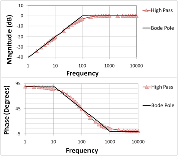
In Figure 1(a), the Bode plots are shown for the one-pole highpass filter function:

where f is the frequency in Hz, and f1 is the pole position in Hz, f1 = 100 Hz in the figure. Using the rules for complex number
Complex number
A complex number is a number consisting of a real part and an imaginary part. Complex numbers extend the idea of the one-dimensional number line to the two-dimensional complex plane by using the number line for the real part and adding a vertical axis to plot the imaginary part...
s, the magnitude of this function is

while the phase is:

Care must be taken that the inverse tangent is set up to return degrees, not radians. On the Bode magnitude plot, decibels are used, and the plotted magnitude is:


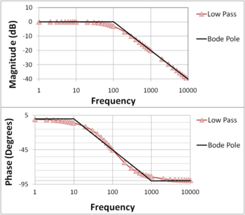
In Figure 1(b), the Bode plots are shown for the one-pole lowpass filter function:

Also shown in Figure 1(a) and 1(b) are the straight-line approximations to the Bode plots that are used in hand analysis, and described later.
The magnitude and phase Bode plots can seldom be changed independently of each other — changing the amplitude response of the system will most likely change the phase characteristics and vice versa. For minimum-phase systems the phase and amplitude characteristics can be obtained from each other with the use of the Hilbert transform
Hilbert transform
In mathematics and in signal processing, the Hilbert transform is a linear operator which takes a function, u, and produces a function, H, with the same domain. The Hilbert transform is named after David Hilbert, who first introduced the operator in order to solve a special case of the...
.
If the transfer function is a rational function
Rational function
In mathematics, a rational function is any function which can be written as the ratio of two polynomial functions. Neither the coefficients of the polynomials nor the values taken by the function are necessarily rational.-Definitions:...
with real poles and zeros, then the Bode plot can be approximated with straight lines. These asymptotic approximations are called straight line Bode plots or uncorrected Bode plots and are useful because they can be drawn by hand following a few simple rules. Simple plots can even be predicted without drawing them.
The approximation can be taken further by correcting the value at each cutoff frequency. The plot is then called a corrected Bode plot.
Rules for hand-made Bode plot
The premise of a Bode plot is that one can consider the log of a function in the form:
as a sum of the logs of its poles and zeros
Zero (complex analysis)
In complex analysis, a zero of a holomorphic function f is a complex number a such that f = 0.-Multiplicity of a zero:A complex number a is a simple zero of f, or a zero of multiplicity 1 of f, if f can be written asf=g\,where g is a holomorphic function g such that g is not zero.Generally, the...
:

This idea is used explicitly in the method for drawing phase diagrams. The method for drawing amplitude plots implicitly uses this idea, but since the log of the amplitude of each pole or zero always starts at zero and only has one asymptote change (the straight lines), the method can be simplified.
Straight-line amplitude plot
Amplitude decibels is usually done using the version. Given a transfer function in the form
where
 and
and  are constants,
  ,
,  , and H is the transfer function:
- at every value of s where
 (a zero), increase the slope of the line by
  per decadeDecade (log scale)One decade is a factor of 10 difference between two numbers measured on a logarithmic scale. It is especially useful when referring to frequencies and when describing frequency response of electronic systems, such as audio amplifiers and filters.-Calculations:The factor-of-ten in a decade can be...
. - at every value of s where
 (a pole), decrease the slope of the line by
  per decade.
 - The initial value of the graph depends on the boundaries. The initial point is found by putting the initial angular frequency ω into the function and finding |H(jω)|.
- The initial slope of the function at the initial value depends on the number and order of zeros and poles that are at values below the initial value, and are found using the first two rules.
To handle irreducible 2nd order polynomials,
 can, in many cases, be approximated as
  .
.Note that zeros and poles happen when ω is equal to a certain
 or
or  . This is because the function in question is the magnitude of H(jω), and since it is a complex function,
  . Thus at any place where there is a zero or pole involving the term
  , the magnitude of that term is
  .
.Corrected amplitude plot
To correct a straight-line amplitude plot:- at every zero, put a point
 above the line,
 - at every pole, put a point
 below the line,
 - draw a smooth curve through those points using the straight lines as asymptotes (lines which the curve approaches).
Note that this correction method does not incorporate how to handle complex values of
 or
or  . In the case of an irreducible polynomial, the best way to correct the plot is to actually calculate the magnitude of the transfer function at the pole or zero corresponding to the irreducible polynomial, and put that dot over or under the line at that pole or zero.
Straight-line phase plot
Given a transfer function in the same form as above:
the idea is to draw separate plots for each pole and zero, then add them up. The actual phase curve is given by
 .
.To draw the phase plot, for each pole and zero:
- if A is positive, start line (with zero slope) at 0 degrees
- if A is negative, start line (with zero slope) at 180 degrees
- at every
 (for stable zeros –
  ), increase the slope by
  degrees per decade, beginning one decade before
  (E.g.:
  )
) - at every
 (for stable poles –
  ), decrease the slope by
  degrees per decade, beginning one decade before
  (E.g.:
  )
) - "unstable" (right half plane) poles and zeros (
 ) have opposite behavior
 - flatten the slope again when the phase has changed by
 degrees (for a zero) or
  degrees (for a pole),
 - After plotting one line for each pole or zero, add the lines together to obtain the final phase plot; that is, the final phase plot is the superposition of each earlier phase plot.
Example
A passive (unity pass band gain) lowpass RC filterRC circuit
A resistor–capacitor circuit ', or RC filter or RC network, is an electric circuit composed of resistors and capacitors driven by a voltage or current source...
, for instance has the following transfer function
Transfer function
A transfer function is a mathematical representation, in terms of spatial or temporal frequency, of the relation between the input and output of a linear time-invariant system. With optical imaging devices, for example, it is the Fourier transform of the point spread function i.e...
expressed in the frequency domain
Frequency domain
In electronics, control systems engineering, and statistics, frequency domain is a term used to describe the domain for analysis of mathematical functions or signals with respect to frequency, rather than time....
:

From the transfer function it can be determined that the cutoff frequency
Cutoff frequency
In physics and electrical engineering, a cutoff frequency, corner frequency, or break frequency is a boundary in a system's frequency response at which energy flowing through the system begins to be reduced rather than passing through.Typically in electronic systems such as filters and...
point fc (in hertz
Hertz
The hertz is the SI unit of frequency defined as the number of cycles per second of a periodic phenomenon. One of its most common uses is the description of the sine wave, particularly those used in radio and audio applications....
) is at the frequency

- or (equivalently) at
 where
where  is the angular cutoff frequency in radians per second.
The transfer function in terms of the angular frequencies becomes:
The above equation is the normalized form of the transfer function. The Bode plot is shown in Figure 1(b) above, and construction of the straight-line approximation is discussed next.
Magnitude plot
The magnitude (in decibelDecibelThe decibel is a logarithmic unit that indicates the ratio of a physical quantity relative to a specified or implied reference level. A ratio in decibels is ten times the logarithm to base 10 of the ratio of two power quantities...
s) of the transfer function above, (normalized and converted to angular frequency form), given by the decibel gain expression :
:
-
-

when plotted versus input frequency on a logarithmic scale, can be approximated by two lines and it forms the asymptotic (approximate) magnitude Bode plot of the transfer function:
- for angular frequencies below
 it is a horizontal line at 0 dB since at low frequencies the
  term is small and can be neglected, making the decibel gain equation above equal to zero,
 - for angular frequencies above
 it is a line with a slope of −20 dB per decade since at high frequencies the
  term dominates and the decibel gain expression above simplifies to
  which is a straight line with a slope of −20 dB per decade.
These two lines meet at the corner frequency. From the plot, it can be seen that for frequencies well below the corner frequency, the circuit has an attenuation of 0 dB, corresponding to a unity pass band gain, i.e. the amplitude of the filter output equals the amplitude of the input. Frequencies above the corner frequency are attenuated – the higher the frequency, the higher the attenuationAttenuationIn physics, attenuation is the gradual loss in intensity of any kind of flux through a medium. For instance, sunlight is attenuated by dark glasses, X-rays are attenuated by lead, and light and sound are attenuated by water.In electrical engineering and telecommunications, attenuation affects the...
.
Phase plot
The phase Bode plot is obtained by plotting the phase angle of the transfer function given by
-

versus , where
  and
and  are the input and cutoff angular frequencies respectively. For input frequencies much lower than corner, the ratio
  is small and therefore the phase angle is close to zero. As the ratio increases the absolute value of the phase increases and becomes –45 degrees when
  . As the ratio increases for input frequencies much greater than the corner frequency, the phase angle asymptotically approaches −90 degrees. The frequency scale for the phase plot is logarithmic.
Normalized plot
The horizontal frequency axis, in both the magnitude and phase plots, can be replaced by the normalized (nondimensional) frequency ratio . In such a case the plot is said to be normalized and units of the frequencies are no longer used since all input frequencies are now expressed as multiples of the cutoff frequency
  .
.
An example with pole and zero
Figures 2-5 further illustrate construction of Bode plots. This example with both a pole and a zero shows how to use superposition. To begin, the components are presented separately.
Figure 2 shows the Bode magnitude plot for a zero and a low-pass pole, and compares the two with the Bode straight line plots. The straight-line plots are horizontal up to the pole (zero) location and then drop (rise) at 20 dB/decade. The second Figure 3 does the same for the phase. The phase plots are horizontal up to a frequency factor of ten below the pole (zero) location and then drop (rise) at 45°/decade until the frequency is ten times higher than the pole (zero) location. The plots then are again horizontal at higher frequencies at a final, total phase change of 90°.
Figure 4 and Figure 5 show how superposition (simple addition) of a pole and zero plot is done. The Bode straight line plots again are compared with the exact plots. The zero has been moved to higher frequency than the pole to make a more interesting example. Notice in Figure 4 that the 20 dB/decade drop of the pole is arrested by the 20 dB/decade rise of the zero resulting in a horizontal magnitude plot for frequencies above the zero location. Notice in Figure 5 in the phase plot that the straight-line approximation is pretty approximate in the region where both pole and zero affect the phase. Notice also in Figure 5 that the range of frequencies where the phase changes in the straight line plot is limited to frequencies a factor of ten above and below the pole (zero) location. Where the phase of the pole and the zero both are present, the straight-line phase plot is horizontal because the 45°/decade drop of the pole is arrested by the overlapping 45°/decade rise of the zero in the limited range of frequencies where both are active contributors to the phase.
Gain margin and phase margin
Bode plots are used to assess the stability of negative feedback amplifiers by finding the gain and phase marginPhase marginIn electronic amplifiers, phase margin is the difference between the phase, measured in degrees, of an amplifier's output signal and 180°, as a function of frequency. The PM is taken as positive at frequencies below where the open-loop phase first crosses 180°, i.e. the signal becomes inverted,...
s of an amplifier. The notion of gain and phase margin is based upon the gain expression for a negative feedback amplifier given by
where AFB is the gain of the amplifier with feedback (the closed-loop gain), β is the feedback factor and AOL is the gain without feedback (the open-loop gain). The gain AOL is a complex function of frequency, with both magnitude and phase.Ordinarily, as frequency increases the magnitude of the gain drops and the phase becomes more negative, although these are only trends and may be reversed in particular frequency ranges. Unusual gain behavior can render the concepts of gain and phase margin inapplicable. Then other methods such as the Nyquist plotNyquist plotA Nyquist plot is a parametric plot of a transfer function used in automatic control and signal processing. The most common use of Nyquist plots is for assessing the stability of a system with feedback. In Cartesian coordinates, the real part of the transfer function is plotted on the X axis. The...
have to be used to assess stability. Examination of this relation shows the possibility of infinite gain (interpreted as instability) if the product βAOL = −1. (That is, the magnitude of βAOL is unity and its phase is −180°, the so-called Barkhausen stability criterionBarkhausen stability criterionThe Barkhausen stability criterion is a mathematical condition to determine when a linear electronic circuit will oscillate. It was put forth in 1921 by German physicist Heinrich Georg Barkhausen...
). Bode plots are used to determine just how close an amplifier comes to satisfying this condition.
Key to this determination are two frequencies. The first, labeled here as f180, is the frequency where the open-loop gain flips sign. The second, labeled here f0dB, is the frequency where the magnitude of the product | β AOL | = 1 (in dB, magnitude 1 is 0 dB). That is, frequency f180 is determined by the condition:

where vertical bars denote the magnitude of a complex number (for example, | a + j b | = [ a2 + b2]1/2 ), and frequency f0dB is determined by the condition:

One measure of proximity to instability is the gain margin. The Bode phase plot locates the frequency where the phase of βAOL reaches −180°, denoted here as frequency f180. Using this frequency, the Bode magnitude plot finds the magnitude of βAOL. If |βAOL|180 = 1, the amplifier is unstable, as mentioned. If |βAOL|180 < 1, instability does not occur, and the separation in dB of the magnitude of |βAOL|180 from |βAOL| = 1 is called the gain margin. Because a magnitude of one is 0 dB, the gain margin is simply one of the equivalent forms: 20 log10( |βAOL|180) = 20 log10( |AOL|180) − 20 log10( 1 / β ).
Another equivalent measure of proximity to instability is the phase marginPhase marginIn electronic amplifiers, phase margin is the difference between the phase, measured in degrees, of an amplifier's output signal and 180°, as a function of frequency. The PM is taken as positive at frequencies below where the open-loop phase first crosses 180°, i.e. the signal becomes inverted,...
. The Bode magnitude plot locates the frequency where the magnitude of |βAOL| reaches unity, denoted here as frequency f0dB. Using this frequency, the Bode phase plot finds the phase of βAOL. If the phase of βAOL( f0dB) > −180°, the instability condition cannot be met at any frequency (because its magnitude is going to be < 1 when f = f180), and the distance of the phase at f0dB in degrees above −180° is called the phase margin.
If a simple yes or no on the stability issue is all that is needed, the amplifier is stable if f0dB < f180. This criterion is sufficient to predict stability only for amplifiers satisfying some restrictions on their pole and zero positions (minimum phaseMinimum phaseIn control theory and signal processing, a linear, time-invariant system is said to be minimum-phase if the system and its inverse are causal and stable....
systems). Although these restrictions usually are met, if they are not another method must be used, such as the Nyquist plotNyquist plotA Nyquist plot is a parametric plot of a transfer function used in automatic control and signal processing. The most common use of Nyquist plots is for assessing the stability of a system with feedback. In Cartesian coordinates, the real part of the transfer function is plotted on the X axis. The...
.
Examples using Bode plots
Figures 6 and 7 illustrate the gain behavior and terminology. For a three-pole amplifier, Figure 6 compares the Bode plot for the gain without feedback (the open-loop gain) AOL with the gain with feedback AFB (the closed-loop gain). See negative feedback amplifier for more detail.
In this example, AOL = 100 dB at low frequencies, and 1 / β = 58 dB. At low frequencies, AFB ≈ 58 dB as well.
Because the open-loop gain AOL is plotted and not the product β AOL, the condition AOL = 1 / β decides f0dB. The feedback gain at low frequencies and for large AOL is AFB ≈ 1 / β (look at the formula for the feedback gain at the beginning of this section for the case of large gain AOL), so an equivalent way to find f0dB is to look where the feedback gain intersects the open-loop gain. (Frequency f0dB is needed later to find the phase margin.)
Near this crossover of the two gains at f0dB, the Barkhausen criteria are almost satisfied in this example, and the feedback amplifier exhibits a massive peak in gain (it would be infinity if β AOL = −1). Beyond the unity gain frequency f0dB, the open-loop gain is sufficiently small that AFB ≈ AOL (examine the formula at the beginning of this section for the case of small AOL).
Figure 7 shows the corresponding phase comparison: the phase of the feedback amplifier is nearly zero out to the frequency f180 where the open-loop gain has a phase of −180°. In this vicinity, the phase of the feedback amplifier plunges abruptly downward to become almost the same as the phase of the open-loop amplifier. (Recall, AFB ≈ AOL for small AOL.)
Comparing the labeled points in Figure 6 and Figure 7, it is seen that the unity gain frequency f0dB and the phase-flip frequency f180 are very nearly equal in this amplifier, f180 ≈ f0dB ≈ 3.332 kHz, which means the gain margin and phase margin are nearly zero. The amplifier is borderline stable.
Figures 8 and 9 illustrate the gain margin and phase margin for a different amount of feedback β. The feedback factor is chosen smaller than in Figure 6 or 7, moving the condition | β AOL | = 1 to lower frequency. In this example, 1 / β = 77 dB, and at low frequencies AFB ≈ 77 dB as well.
Figure 8 shows the gain plot. From Figure 8, the intersection of 1 / β and AOL occurs at f0dB = 1 kHz. Notice that the peak in the gain AFB near f0dB is almost gone.The critical amount of feedback where the peak in the gain just disappears altogether is the maximally flat or Butterworth design.
Figure 9 is the phase plot. Using the value of f0dB = 1 kHz found above from the magnitude plot of Figure 8, the open-loop phase at f0dB is −135°, which is a phase margin of 45° above −180°.
Using Figure 9, for a phase of −180° the value of f180 = 3.332 kHz (the same result as found earlier, of courseThe frequency where the open-loop gain flips sign f180 does not change with a change in feedback factor; it is a property of the open-loop gain. The value of the gain at f180 also does not change with a change in β. Therefore, we could use the previous values from Figures 6 and 7. However, for clarity the procedure is described using only Figures 8 and 9.). The open-loop gain from Figure 8 at f180 is 58 dB, and 1 / β = 77 dB, so the gain margin is 19 dB.
Stability is not the sole criterion for amplifier response, and in many applications a more stringent demand than stability is good step response. As a rule of thumbRule of thumbA rule of thumb is a principle with broad application that is not intended to be strictly accurate or reliable for every situation. It is an easily learned and easily applied procedure for approximately calculating or recalling some value, or for making some determination...
, good step response requires a phase margin of at least 45°, and often a margin of over 70° is advocated, particularly where component variation due to manufacturing tolerances is an issue. See also the discussion of phase margin in the step response article.
Bode plotter
The Bode plotter is an electronic instrument resembling an oscilloscope OscilloscopeAn oscilloscope is a type of electronic test instrument that allows observation of constantly varying signal voltages, usually as a two-dimensional graph of one or more electrical potential differences using the vertical or 'Y' axis, plotted as a function of time,...
, which produces a Bode diagram, or a graph, of a circuit's voltage gain or phase shift plotted against frequencyFrequencyFrequency is the number of occurrences of a repeating event per unit time. It is also referred to as temporal frequency.The period is the duration of one cycle in a repeating event, so the period is the reciprocal of the frequency...
in a feedback control system or a filter. An example of this is shown in Figure 10. It is extremely useful for analyzing and testing filters and the stability of feedbackFeedbackFeedback describes the situation when output from an event or phenomenon in the past will influence an occurrence or occurrences of the same Feedback describes the situation when output from (or information about the result of) an event or phenomenon in the past will influence an occurrence or...
control systems, through the measurement of corner (cutoff) frequencies and gain and phase margins.
This is identical to the function performed by a vector network analyzerNetwork analyzer (electrical)A network analyzer is an instrument that measures the network parameters of electrical networks. Today, network analyzers commonly measure s–parameters because reflection and transmission of electrical networks are easy to measure at high frequencies, but there are other network parameter...
, but the network analyzer is typically used at much higher frequencies.
For education/research purposes, plotting Bode diagrams for given transfer functions facilitates better understanding and getting faster results (see external links).
Related plots
Two related plots that display the same data in different coordinate systems are the Nyquist plotNyquist plotA Nyquist plot is a parametric plot of a transfer function used in automatic control and signal processing. The most common use of Nyquist plots is for assessing the stability of a system with feedback. In Cartesian coordinates, the real part of the transfer function is plotted on the X axis. The...
and the Nichols plot. These are parametric plots, with frequency as the input and magnitude and phase of the frequency response as the output. The Nyquist plot displays these in polar coordinates, with magnitude mapping to radius and phase to argument (angle). The Nichols plot displays these in rectangular coordinates, on the log scale.
See also
- Nichols plot
- Analog signal processingAnalog signal processingAnalog signal processing is any signal processing conducted on analog signals by analog means. "Analog" indicates something that is mathematically represented as a set of continuous values. This differs from "digital" which uses a series of discrete quantities to represent signal...
- Phase marginPhase marginIn electronic amplifiers, phase margin is the difference between the phase, measured in degrees, of an amplifier's output signal and 180°, as a function of frequency. The PM is taken as positive at frequencies below where the open-loop phase first crosses 180°, i.e. the signal becomes inverted,...
- Bode's sensitivity integralBode's sensitivity integralBode's sensitivity integral, discovered by Hendrik Wade Bode, is a formula that quantifies some of the limitations in feedback control of linear parameter invariant systems. Let L be the loop transfer function and S be the sensitivity function...
- Electrochemical impedance spectroscopy
External links
- Explanation of Bode plots with movies and examples
- How to draw piecewise asymptotic Bode plots
- Summarized drawing rules (PDF)
- Bode plot applet - Accepts transfer function coefficients as input, and calculates magnitude and phase response
- Circuit analysis in electrochemistry
- Tim Green: Operational amplifier stability Includes some Bode plot introduction
- Gnuplot code for generating Bode plot: DIN-A4 printing template (pdf)
-
- for angular frequencies below
-
-
