
Gravitational lensing formalism
Encyclopedia
In general relativity
, a point mass deflects a light ray with impact parameter
 by an angle
  . A naïve application of Newtonian gravity can yield exactly half this value, where the light ray is assumed as a massed particle and scattered by the gravitational potential well.
In situations where General Relativity can be approximated by linearized gravity
, the deflection due to a spatially extended mass can be written simply as a vector sum over point masses. In the continuum limit, this becomes an integral over the density , and if the deflection is small we can approximate the gravitational potential along the deflected trajectory by the potential along the undeflected trajectory, as in the Born approximation
in Quantum Mechanics. The deflection is then
where is the line-of-sight coordinate, and
  is the vector impact parameter of the actual ray path from the infinitesimal mass
  located at the coordinates
  .
.
where is a vector in the plane of the sky. The deflection angle is then
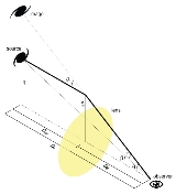
 As shown in the diagram on the right, the difference between the unlensed angular position
  and the observed position
  is this deflection angle, reduced by a ratio of distances, described as the lens equation
where is the distance from the lens to the source
  is the distance from the observer to the source, and
  is the distance from the observer to the lens. For extragalactic lenses, these must be angular diameter distances.
In strong gravitational lensing, this equation can have multiple solutions, because a single source at can be lensed into multiple images.

and the critical surface density (not to be confused with the critical density of the universe)
The reduced deflection angle can now be written as
We can also define the deflection potential
such that the scaled deflection angle is just the gradient
of the potential and the convergence is half the Laplacian of the potential:


The deflection potential can also be written as a scaled projection of the Newtonian gravitational potential of the lens
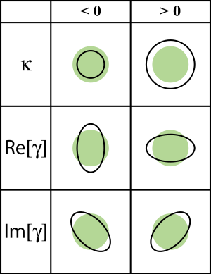
where is the Kronecker delta. Because the matrix of second derivatives must be symmetric, the Jacobian can be decomposed into a diagonal term involving the convergence and a trace-free term involving the shear
where is the angle between
  and the x-axis. The term involving the convergence magnifies the image by increasing its size while conserving surface brightness. The term involving the shear stretches the image tangentially around the lens, as discussed in weak lensing observables.
The shear defined here is not equivalent to the shear traditionally defined in mathematics, though both stretch an image non-uniformly.
There is an alternative way of deriving the lens equation, starting from the photon arrival time (Fermat surface)
where is the time to travel an infinitesimal line element along the source-observer straight line in vacuum, which is
then corrected by the factor
to get the line element along the bended path with a varying small pitch angle
  , and the refraction index
n for the "aether", i.e., the gravitational field. The last can be obtained from the fact that a photon travels on a null geodesic of a weakly-perturbed static Minkowski universe

where the uneven gravitational potential drives a changing the speed of light
So the refraction index

The refraction index greater than unity because of the negative gravitational potential .
.
Put these together and keep the leading terms we have the time arrival surface
The first term is the straight path travel time, the second term is the extra geometric path, and the third is the gravitational delay.
Make the triangle approximation that for the path between the observer and the lens,
and for the path between the lens and the source.
The geometric delay term becomes
So the Fermat surface becomes
where is so-called dimensionless time delay, and the 2D lensing potential

The images lie at the extrema of this surface, so the variation of t with is zero,
which is the lens equation. Take the Poisson's equation for 3D potential
and we find the 2D lensing potential

Here we assumed the lens is a collection of point masses at angular coordinates
  and distances
  .
.
Use for very small x we find
One can compute the convergence by applying the 2D Laplacian of the 2D lensing potential

in agreement with earlier definition as the ratio of projected density with the critical density.
Here we used and
and  .
.
We can also confirm the previously-defined reduced deflection angle
where is the so-called Einstein angular radius of a point lens Mi. For a single point lens at the origin we recover the standard result
that there will be two images at the two solutions of the essentially quadratic equation

The amplification matrix can be obtained by double derivatives of the dimensionless time delay
where we have define the derivatives

which takes the meaning of convergence and shear. The amplification is the inverse of the Jacobian
where a positive A means either a maxima or a minima, and a negative A means a saddle point in the arrival surface.
For a single point lens, one can show (albeit a lengthy calculation) that
So the amplification of a point lens is given by

Note A diverges for images at the Einstein radius .
.
In cases there are multiple point lenses plus a smooth background of (dark) particles of surface density , the time arrival surface is
To compute the amplification, e.g., at the origin (0,0), due to identical point masses distributed at
we have to add up the total shear, and include an convergence of the smooth background,
This generally creates a network of critical curves, lines connecting image points of infinite amplification.
This approach assumes the universe is well described by a Newtonian-perturbed FRW metric, but it makes no other assumptions about the distribution of the lensing mass.
As in the thin-lens case, the effect can be written as a mapping from the unlensed angular position to the lensed position
  . The Jacobian of the transform can be written as an integral over the gravitational potential
  along the line of sight
where is the comoving distance
, are the transverse distances, and
is the lensing kernel, which defines the efficiency of lensing for a distribution of sources .
.
The Jacobian can be decomposed into convergence and shear terms just as with the thin-lens case, and in the limit of a lens that is both thin and weak, their physical interpretations are the same.
, the Jacobian is mapped out by observing the effect of the shear on the ellipticities of background galaxies. This effect is purely statistical; the shape of any galaxy will be dominated by its random, unlensed shape, but lensing will produce a spatially coherent distortion of these shapes.
 , where
  is the axis ratio of the ellipse
. In weak gravitational lensing
, two different definitions are commonly used, and both are complex quantities which specify both the axis ratio and the position angle :
:
Like the traditional ellipticity, the magnitudes of both of these quantities range from 0 (circular) to 1 (a line segment). The position angle is encoded in the complex phase, but because of the factor of 2 in the trigonometric arguments, ellipticity is invariant under a rotation of 180 degrees. This is to be expected; an ellipse is unchanged by a 180° rotation. Taken as imaginary and real parts, the real part of the complex ellipticity describes the elongation along the coordinate axes, while the imaginary part describes the elongation at 45° from the axes.
The ellipticity is often written as a two-component vector instead of a complex number, though it is not a true vector
with regard to transforms:
Real astronomical background sources are not perfect ellipses. Their ellipticities can be measured by finding a best-fit elliptical model to the data, or by measuring the second moments of the image about some centroid

The complex ellipticities are then
This can be used to relate the second moments to traditional ellipse parameters:
and in reverse:

The unweighted second moments above are problematic in the presence of noise, neighboring objects, or extended galaxy profiles, so it is typical to use apodized
moments instead:
Here is a weight function that typically goes to zero or quickly approaches zero at some finite radius.
Image moments cannot generally be used to measure the ellipticity of galaxies without correcting for observational effects, particularly the point spread function
.
 and convergence
  .
.
Acting on a circular background source with radius , lensing generates an ellipse with major and minor axes


as long as the shear and convergence do not change appreciably over the size of the source (in that case, the lensed image is not an ellipse). Galaxies are not intrinsically circular, however, so it is necessary to quantify the effect of lensing on a non-zero ellipticity.
We can define the complex shear in analogy to the complex ellipticities defined above

as well as the reduced shear

The lensing Jacobian can now be written as

For a reduced shear and unlensed complex ellipticities
  and
and  , the lensed ellipticities are

In the weak lensing limit, and
and  , so
, so
If we can assume that the sources are randomly oriented, their complex ellipticities average to zero, so
 and
and  .
.
This is the principal equation of weak lensing: the average ellipticity of background galaxies is a direct measure of the shear induced by foreground mass.
, lensing does change the apparent solid angle
of a source. The amount of magnification
is given by the ratio of the image area to the source area. For a circularly symmetric
lens, the magnification factor μ is given by

In terms of convergence and shear
For this reason, the Jacobian is also known as the "inverse magnification matrix".
The reduced shear is invariant with the scaling of the Jacobian by a scalar
  , which is equivalent to the transformations

and
 .
.
Thus, can only be determined up to a transformation
  , which is known as the "mass sheet degeneracy." In principle, this degeneracy can be broken if an independent measurement of the magnification is available because the magnification is not invariant under the aforementioned degeneracy transformation. Specifically,
  scales with
  as
as  .
.
General relativity
General relativity or the general theory of relativity is the geometric theory of gravitation published by Albert Einstein in 1916. It is the current description of gravitation in modern physics...
, a point mass deflects a light ray with impact parameter
Impact parameter
The impact parameter b is defined as the perpendicular distance between the path of a projectile and the center of the field U created by an object that the projectile is approaching...
by an angle . A naïve application of Newtonian gravity can yield exactly half this value, where the light ray is assumed as a massed particle and scattered by the gravitational potential well.In situations where General Relativity can be approximated by linearized gravity
Linearized gravity
Linearized gravity is an approximation scheme in general relativity in which the nonlinear contributions from the spacetime metric are ignored, simplifying the study of many problems while still producing useful approximate results.-The method:...
, the deflection due to a spatially extended mass can be written simply as a vector sum over point masses. In the continuum limit, this becomes an integral over the density
, and if the deflection is small we can approximate the gravitational potential along the deflected trajectory by the potential along the undeflected trajectory, as in the Born approximationBorn approximation
In scattering theory and, in particular in quantum mechanics, the Born approximation consists of taking the incident field in place of the total field as the driving field at each point in the scatterer. Born approximation is named after Max Born, winner of the 1954 Nobel Prize for physics.It is...
in Quantum Mechanics. The deflection is then
where
is the line-of-sight coordinate, and is the vector impact parameter of the actual ray path from the infinitesimal mass located at the coordinates .Thin lens approximation
In the limit of a "thin lens", where the distances between the source, lens, and observer are much larger than the size of the lens (this is almost always true for astronomical objects), we can define the projected mass densitywhere
is a vector in the plane of the sky. The deflection angle is then and the observed position is this deflection angle, reduced by a ratio of distances, described as the lens equationwhere
is the distance from the lens to the source is the distance from the observer to the source, and is the distance from the observer to the lens. For extragalactic lenses, these must be angular diameter distances.In strong gravitational lensing, this equation can have multiple solutions, because a single source at
can be lensed into multiple images.Convergence and deflection potential
It is convenient to define the convergenceand the critical surface density (not to be confused with the critical density of the universe)
The reduced deflection angle
can now be written asWe can also define the deflection potential
such that the scaled deflection angle is just the gradient
Gradient
In vector calculus, the gradient of a scalar field is a vector field that points in the direction of the greatest rate of increase of the scalar field, and whose magnitude is the greatest rate of change....
of the potential and the convergence is half the Laplacian of the potential:
The deflection potential can also be written as a scaled projection of the Newtonian gravitational potential
of the lensLensing Jacobian
The Jacobian between the unlensed and lensed coordinate systems iswhere
is the Kronecker delta. Because the matrix of second derivatives must be symmetric, the Jacobian can be decomposed into a diagonal term involving the convergence and a trace-free term involving the shear where
is the angle between and the x-axis. The term involving the convergence magnifies the image by increasing its size while conserving surface brightness. The term involving the shear stretches the image tangentially around the lens, as discussed in weak lensing observables.The shear defined here is not equivalent to the shear traditionally defined in mathematics, though both stretch an image non-uniformly.
Fermat Surface
There is an alternative way of deriving the lens equation, starting from the photon arrival time (Fermat surface)
where
is the time to travel an infinitesimal line element along the source-observer straight line in vacuum, which isthen corrected by the factor
to get the line element along the bended path
with a varying small pitch angle , and the refraction indexn for the "aether", i.e., the gravitational field. The last can be obtained from the fact that a photon travels on a null geodesic of a weakly-perturbed static Minkowski universe
where the uneven gravitational potential
drives a changing the speed of lightSo the refraction index
The refraction index greater than unity because of the negative gravitational potential
.Put these together and keep the leading terms we have the time arrival surface
The first term is the straight path travel time, the second term is the extra geometric path, and the third is the gravitational delay.
Make the triangle approximation that
for the path between the observer and the lens,and
for the path between the lens and the source.The geometric delay term becomes
So the Fermat surface becomes
where
is so-called dimensionless time delay, and the 2D lensing potentialThe images lie at the extrema of this surface, so the variation of t with
is zero,which is the lens equation. Take the Poisson's equation for 3D potential
and we find the 2D lensing potential
Here we assumed the lens is a collection of point masses
at angular coordinates and distances .Use
for very small x we findOne can compute the convergence by applying the 2D Laplacian of the 2D lensing potential
in agreement with earlier definition
as the ratio of projected density with the critical density.Here we used
and .We can also confirm the previously-defined reduced deflection angle
where
is the so-called Einstein angular radius of a point lens Mi. For a single point lens at the origin we recover the standard resultthat there will be two images at the two solutions of the essentially quadratic equation
The amplification matrix can be obtained by double derivatives of the dimensionless time delay
where we have define the derivatives
which takes the meaning of convergence and shear. The amplification is the inverse of the Jacobian
where a positive A means either a maxima or a minima, and a negative A means a saddle point in the arrival surface.
For a single point lens, one can show (albeit a lengthy calculation) that
So the amplification of a point lens is given by
Note A diverges for images at the Einstein radius
.In cases there are multiple point lenses plus a smooth background of (dark) particles of surface density
, the time arrival surface isTo compute the amplification, e.g., at the origin (0,0), due to identical point masses distributed at
we have to add up the total shear, and include an convergence of the smooth background,
This generally creates a network of critical curves, lines connecting image points of infinite amplification.
General weak lensing
In weak lensing by large scale structure, the thin-lens approximation may break down, and low-density extended structures may not be well approximated by multiple thin-lens planes. In this case, the deflection can be derived by instead assuming that the gravitational potential is slowly varying everywhere (for this reason, this approximation is not valid for strong lensing).This approach assumes the universe is well described by a Newtonian-perturbed FRW metric, but it makes no other assumptions about the distribution of the lensing mass.
As in the thin-lens case, the effect can be written as a mapping from the unlensed angular position
to the lensed position . The Jacobian of the transform can be written as an integral over the gravitational potential along the line of sightwhere
is the comoving distanceComoving distance
In standard cosmology, comoving distance and proper distance are two closely related distance measures used by cosmologists to define distances between objects...
,
are the transverse distances, andis the lensing kernel, which defines the efficiency of lensing for a distribution of sources
.The Jacobian
can be decomposed into convergence and shear terms just as with the thin-lens case, and in the limit of a lens that is both thin and weak, their physical interpretations are the same.Weak lensing observables
In weak gravitational lensingWeak gravitational lensing
While the presence of any mass bends the path of light passing near it, this effect rarely produces the giant arcs and multiple images associated with strong gravitational lensing. Most lines of sight in the universe are thoroughly in the weak lensing regime, in which the deflection is impossible...
, the Jacobian is mapped out by observing the effect of the shear on the ellipticities of background galaxies. This effect is purely statistical; the shape of any galaxy will be dominated by its random, unlensed shape, but lensing will produce a spatially coherent distortion of these shapes.
Measures of ellipticity
In most fields of astronomy, the ellipticity is defined as, where is the axis ratio of the ellipseEllipse
In geometry, an ellipse is a plane curve that results from the intersection of a cone by a plane in a way that produces a closed curve. Circles are special cases of ellipses, obtained when the cutting plane is orthogonal to the cone's axis...
. In weak gravitational lensing
Weak gravitational lensing
While the presence of any mass bends the path of light passing near it, this effect rarely produces the giant arcs and multiple images associated with strong gravitational lensing. Most lines of sight in the universe are thoroughly in the weak lensing regime, in which the deflection is impossible...
, two different definitions are commonly used, and both are complex quantities which specify both the axis ratio and the position angle
:Like the traditional ellipticity, the magnitudes of both of these quantities range from 0 (circular) to 1 (a line segment). The position angle is encoded in the complex phase, but because of the factor of 2 in the trigonometric arguments, ellipticity is invariant under a rotation of 180 degrees. This is to be expected; an ellipse is unchanged by a 180° rotation. Taken as imaginary and real parts, the real part of the complex ellipticity describes the elongation along the coordinate axes, while the imaginary part describes the elongation at 45° from the axes.
The ellipticity is often written as a two-component vector instead of a complex number, though it is not a true vector
Coordinate vector
In linear algebra, a coordinate vector is an explicit representation of a vector in an abstract vector space as an ordered list of numbers or, equivalently, as an element of the coordinate space Fn....
with regard to transforms:
Real astronomical background sources are not perfect ellipses. Their ellipticities can be measured by finding a best-fit elliptical model to the data, or by measuring the second moments of the image about some centroid
Centroid
In geometry, the centroid, geometric center, or barycenter of a plane figure or two-dimensional shape X is the intersection of all straight lines that divide X into two parts of equal moment about the line. Informally, it is the "average" of all points of X...
The complex ellipticities are then
This can be used to relate the second moments to traditional ellipse parameters:
and in reverse:
The unweighted second moments above are problematic in the presence of noise, neighboring objects, or extended galaxy profiles, so it is typical to use apodized
Apodization
Apodization literally means "removing the foot". It is the technical term for changing the shape of a mathematical function, an electrical signal, an optical transmission or a mechanical structure.- Apodization in signal processing :...
moments instead:
Here
is a weight function that typically goes to zero or quickly approaches zero at some finite radius.Image moments cannot generally be used to measure the ellipticity of galaxies without correcting for observational effects, particularly the point spread function
Point spread function
The point spread function describes the response of an imaging system to a point source or point object. A more general term for the PSF is a system's impulse response, the PSF being the impulse response of a focused optical system. The PSF in many contexts can be thought of as the extended blob...
.
Shear and reduced shear
Recall that the lensing Jacobian can be decomposed into shear and convergence .Acting on a circular background source with radius
, lensing generates an ellipse with major and minor axesas long as the shear and convergence do not change appreciably over the size of the source (in that case, the lensed image is not an ellipse). Galaxies are not intrinsically circular, however, so it is necessary to quantify the effect of lensing on a non-zero ellipticity.
We can define the complex shear in analogy to the complex ellipticities defined above
as well as the reduced shear
The lensing Jacobian can now be written as
For a reduced shear
and unlensed complex ellipticities and , the lensed ellipticities areIn the weak lensing limit,
and , soIf we can assume that the sources are randomly oriented, their complex ellipticities average to zero, so
and .This is the principal equation of weak lensing: the average ellipticity of background galaxies is a direct measure of the shear induced by foreground mass.
Magnification
While gravitational lensing preserves surface brightness, as dictated by Liouville's theoremLiouville's theorem
Liouville's theorem has various meanings, all mathematical results named after Joseph Liouville:*In complex analysis, see Liouville's theorem ; there is also a related theorem on harmonic functions....
, lensing does change the apparent solid angle
Solid angle
The solid angle, Ω, is the two-dimensional angle in three-dimensional space that an object subtends at a point. It is a measure of how large that object appears to an observer looking from that point...
of a source. The amount of magnification
Magnification
Magnification is the process of enlarging something only in appearance, not in physical size. This enlargement is quantified by a calculated number also called "magnification"...
is given by the ratio of the image area to the source area. For a circularly symmetric
Symmetry
Symmetry generally conveys two primary meanings. The first is an imprecise sense of harmonious or aesthetically pleasing proportionality and balance; such that it reflects beauty or perfection...
lens, the magnification factor μ is given by
In terms of convergence and shear
For this reason, the Jacobian
is also known as the "inverse magnification matrix".The reduced shear is invariant with the scaling of the Jacobian
by a scalar , which is equivalent to the transformationsand
.Thus,
can only be determined up to a transformation , which is known as the "mass sheet degeneracy." In principle, this degeneracy can be broken if an independent measurement of the magnification is available because the magnification is not invariant under the aforementioned degeneracy transformation. Specifically, scales with as .