CMA-ES
Encyclopedia
CMA-ES stands for Covariance Matrix Adaptation Evolution Strategy. Evolution strategies (ES) are stochastic
, derivative
-free methods for numerical optimization of non-linear or non-convex
continuous optimization
problems. They belong to the class of evolutionary algorithms and evolutionary computation
. An evolutionary algorithm
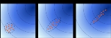
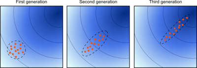
is broadly based on the principle of biological evolution, namely the repeated interplay of variation (via mutation and recombination) and selection: in each generation (iteration) new individuals (candidate solutions, denoted as ) are generated by variation, usually in a stochastic way, and then some individuals are selected for the next generation based on their fitness or objective function value
  . Like this, over the generation sequence, individuals with better and better
  -values are generated.
In an evolution strategy
, new candidate solutions are sampled according to a multivariate normal distribution in the . Pairwise dependencies between the variables in this distribution are described by a covariance matrix
. The covariance matrix adaptation (CMA) is a method to update the covariance matrix
of this distribution. This is particularly useful, if the function is ill-conditioned.
Adaptation of the covariance matrix
amounts to learning a second order model of the underlying objective function similar to the approximation of the inverse Hessian matrix
in the Quasi-Newton method
in classical optimization
. In contrast to most classical methods, fewer assumptions on the nature of the underlying objective function are made. Only the ranking between candidate solutions is exploited for learning the sample distribution and neither derivatives nor even the function values themselves are required by the method.
 Two main principles for the adaptation of parameters of the search distribution are exploited in the CMA-ES algorithm.
First, a maximum-likelihood principle, based on the idea to increase the probability of successful candidate solutions and search steps. The mean of the distribution is updated such that the likelihood
of previously successful candidate solutions is maximized. The covariance matrix
of the distribution is updated (incrementally) such that the likelihood of previously successful search steps is increased. Both updates can be interpreted as a natural gradient descent. Also, in consequence, the CMA conducts an iterated principal components analysis
of successful search steps while retaining all principal axes. Estimation of distribution algorithms
and the Cross-Entropy Method
are based on very similar ideas, but estimate (non-incrementally) the covariance matrix by maximizing the likelihood of successful solution points instead of successful search steps.
Second, two paths of the time evolution of the distribution mean of the strategy are recorded, called search or evolution paths. These paths contain significant information about the correlation between consecutive steps. Specifically, if consecutive steps are taken in a similar direction, the evolution paths become long. The evolution paths are exploited in two ways. One path is used for the covariance matrix adaptation procedure in place of single successful search steps and facilitates a possibly much faster variance increase of favorable directions. The other path is used to conduct an additional step-size control. This step-size control aims to make consecutive movements of the distribution mean orthogonal in expectation. The step-size control effectively prevents premature convergence
yet allowing fast convergence to an optimum.
of the algorithm looks as follows.
The order of the five update assignments is relevant. In the following, the update equations for the five state variables is specified.
Given are the search space dimension and the iteration step
  . The five state variables are
The iteration starts with sampling candidate solutions
  from a multivariate normal distribution
  , i.e.
for
Stochastic
Stochastic refers to systems whose behaviour is intrinsically non-deterministic. A stochastic process is one whose behavior is non-deterministic, in that a system's subsequent state is determined both by the process's predictable actions and by a random element. However, according to M. Kac and E...
, derivative
Derivative
In calculus, a branch of mathematics, the derivative is a measure of how a function changes as its input changes. Loosely speaking, a derivative can be thought of as how much one quantity is changing in response to changes in some other quantity; for example, the derivative of the position of a...
-free methods for numerical optimization of non-linear or non-convex
Convex function
In mathematics, a real-valued function f defined on an interval is called convex if the graph of the function lies below the line segment joining any two points of the graph. Equivalently, a function is convex if its epigraph is a convex set...
continuous optimization
Continuous optimization
Continuous optimization is a branch of optimization in applied mathematics.As opposed to discrete optimization, the variables used in the objective function can assume real values, e.g., values from intervals of the real line....
problems. They belong to the class of evolutionary algorithms and evolutionary computation
Evolutionary computation
In computer science, evolutionary computation is a subfield of artificial intelligence that involves combinatorial optimization problems....
. An evolutionary algorithm
Evolutionary algorithm
In artificial intelligence, an evolutionary algorithm is a subset of evolutionary computation, a generic population-based metaheuristic optimization algorithm. An EA uses some mechanisms inspired by biological evolution: reproduction, mutation, recombination, and selection...
is broadly based on the principle of biological evolution, namely the repeated interplay of variation (via mutation and recombination) and selection: in each generation (iteration) new individuals (candidate solutions, denoted as
) are generated by variation, usually in a stochastic way, and then some individuals are selected for the next generation based on their fitness or objective function value . Like this, over the generation sequence, individuals with better and better -values are generated.In an evolution strategy
Evolution strategy
In computer science, evolution strategy is an optimization technique based on ideas of adaptation and evolution. It belongs to the general class of evolutionary computation or artificial evolution methodologies.-History:...
, new candidate solutions are sampled according to a multivariate normal distribution in the
. Pairwise dependencies between the variables in this distribution are described by a covariance matrixCovariance matrix
In probability theory and statistics, a covariance matrix is a matrix whose element in the i, j position is the covariance between the i th and j th elements of a random vector...
. The covariance matrix adaptation (CMA) is a method to update the covariance matrix
Covariance matrix
In probability theory and statistics, a covariance matrix is a matrix whose element in the i, j position is the covariance between the i th and j th elements of a random vector...
of this distribution. This is particularly useful, if the function
is ill-conditioned.Adaptation of the covariance matrix
Covariance matrix
In probability theory and statistics, a covariance matrix is a matrix whose element in the i, j position is the covariance between the i th and j th elements of a random vector...
amounts to learning a second order model of the underlying objective function similar to the approximation of the inverse Hessian matrix
Hessian matrix
In mathematics, the Hessian matrix is the square matrix of second-order partial derivatives of a function; that is, it describes the local curvature of a function of many variables. The Hessian matrix was developed in the 19th century by the German mathematician Ludwig Otto Hesse and later named...
in the Quasi-Newton method
Quasi-Newton method
In optimization, quasi-Newton methods are algorithms for finding local maxima and minima of functions. Quasi-Newton methods are based on...
in classical optimization
Optimization (mathematics)
In mathematics, computational science, or management science, mathematical optimization refers to the selection of a best element from some set of available alternatives....
. In contrast to most classical methods, fewer assumptions on the nature of the underlying objective function are made. Only the ranking between candidate solutions is exploited for learning the sample distribution and neither derivatives nor even the function values themselves are required by the method.
Principles
First, a maximum-likelihood principle, based on the idea to increase the probability of successful candidate solutions and search steps. The mean of the distribution is updated such that the likelihood
Likelihood
Likelihood is a measure of how likely an event is, and can be expressed in terms of, for example, probability or odds in favor.-Likelihood function:...
of previously successful candidate solutions is maximized. The covariance matrix
Covariance matrix
In probability theory and statistics, a covariance matrix is a matrix whose element in the i, j position is the covariance between the i th and j th elements of a random vector...
of the distribution is updated (incrementally) such that the likelihood of previously successful search steps is increased. Both updates can be interpreted as a natural gradient descent. Also, in consequence, the CMA conducts an iterated principal components analysis
Principal components analysis
Principal component analysis is a mathematical procedure that uses an orthogonal transformation to convert a set of observations of possibly correlated variables into a set of values of uncorrelated variables called principal components. The number of principal components is less than or equal to...
of successful search steps while retaining all principal axes. Estimation of distribution algorithms
Estimation of Distribution Algorithms
Estimation of Distribution Algorithms , sometimes called Probabilistic Model-Building Genetic Algorithms , are an outgrowth of genetic algorithms. In a genetic algorithm, a population of candidate solutions to a problem is maintained as part of the search for an optimum solution. This population is...
and the Cross-Entropy Method
Cross-entropy method
The cross-entropy method attributed to Reuven Rubinstein is a general Monte Carlo approach tocombinatorial and continuous multi-extremal optimization and importance sampling.The method originated from the field of rare event simulation, where...
are based on very similar ideas, but estimate (non-incrementally) the covariance matrix by maximizing the likelihood of successful solution points instead of successful search steps.
Second, two paths of the time evolution of the distribution mean of the strategy are recorded, called search or evolution paths. These paths contain significant information about the correlation between consecutive steps. Specifically, if consecutive steps are taken in a similar direction, the evolution paths become long. The evolution paths are exploited in two ways. One path is used for the covariance matrix adaptation procedure in place of single successful search steps and facilitates a possibly much faster variance increase of favorable directions. The other path is used to conduct an additional step-size control. This step-size control aims to make consecutive movements of the distribution mean orthogonal in expectation. The step-size control effectively prevents premature convergence
Premature convergence
In genetic algorithms, the term of premature convergence means that a population for an optimization problem converged too early, resulting in being suboptimal. In this context, the parental solutions, through the aid of genetic operators, are not able to generate offsprings that are superior to...
yet allowing fast convergence to an optimum.
Algorithm
In the following the most commonly used (μ/μw, λ)-CMA-ES is outlined, where in each iteration step a weighted combination of the μ best out of λ new candidate solutions is used to update the distribution parameters. The main loop consists of three main parts: 1) sampling of new solutions, 2) re-ordering of the sampled solutions based on their fitness, 3) update of the internal state variables based on the re-ordered samples. A pseudocodePseudocode
In computer science and numerical computation, pseudocode is a compact and informal high-level description of the operating principle of a computer program or other algorithm. It uses the structural conventions of a programming language, but is intended for human reading rather than machine reading...
of the algorithm looks as follows.
set  // number of samples per iteration, at least two, generally > 4
initialize  ,
,  ,
,  ,
,  ,
,  // initialize state variables
while not terminate // iterate
for  in
in  // sample
  new solutions and evaluate them
 = sample_multivariate_normal(mean=
 , covariance_matrix=
 )
)
 = fitness(
 )
)
 ←
←  with
with  = argsort(
 ,
,  ) // sort solutions
 =
=  // we need later
  and
and 
 ← update_m
 // move mean to better solutions
 ← update_ps
 // update isotropic evolution path
 ← update_pc

 // update anisotropic evolution path
 ← update_C


 // update covariance matrix
 ← update_sigma
 // update step-size using isotropic path length
return  or
or 
The order of the five update assignments is relevant. In the following, the update equations for the five state variables is specified.
Given are the search space dimension
and the iteration step . The five state variables are-
 , the distribution mean and current favorite solution to the optimization problem,
-
 , the step-size,
-
 , a symmetric and positive definitePositive-definite matrixIn linear algebra, a positive-definite matrix is a matrix that in many ways is analogous to a positive real number. The notion is closely related to a positive-definite symmetric bilinear form ....
 covariance matrixCovariance matrixIn probability theory and statistics, a covariance matrix is a matrix whose element in the i, j position is the covariance between the i th and j th elements of a random vector...
with and
and
-
 , two evolution paths, initially set to the zero vector.
The iteration starts with sampling
candidate solutions from a multivariate normal distribution , i.e.for
-
-

The second line suggests the interpretation as perturbation (mutation) of the current favorite solution vector (the distribution mean vector). The candidate solutions
  are evaluated on the objective function
  to be minimized. Denoting the
  -sorted candidate solutions as
-

the new mean value is computed as
-
-

where the positive (recombination) weights sum to one. Typically,
  and the weights are chosen such that
  . The only feedback used from the objective function here and in the following is an ordering of the sampled candidate solutions due to the indices
  .
.
The step-size is updated using cumulative step-size adaptation (CSA), sometimes also denoted as path length control. The evolution path (or search path)
  is updated first.
-
-

-
-

where
-
 is the backward time horizon for the evolution path
  and larger than one,
-
 is the variance effective selection mass and
  by definition of
  ,
,
-
 is the unique symmetric square rootSquare root of a matrixIn mathematics, the square root of a matrix extends the notion of square root from numbers to matrices. A matrix B is said to be a square root of A if the matrix product B · B is equal to A.-Properties:...
of the inverse of , and
, and
-
 is the damping parameter usually close to one. For
  or
or  the step-size remains unchanged.
The step-size is increased if and only if
  is larger than the expected valueExpected valueIn probability theory, the expected value of a random variable is the weighted average of all possible values that this random variable can take on...
-

and decreased if it is smaller. For this reason, the step-size update tends to make consecutive steps -conjugate, in that after the adaptation has been successful
  .
.
Finally, the covariance matrixCovariance matrixIn probability theory and statistics, a covariance matrix is a matrix whose element in the i, j position is the covariance between the i th and j th elements of a random vector...
is updated, where again the respective evolution path is updated first.
-
-

-
-

where denotes the transpose and
-
 is the backward time horizon for the evolution path
  and larger than one,
-
 and the indicator function
  evaluates to one iffIf and only ifIn logic and related fields such as mathematics and philosophy, if and only if is a biconditional logical connective between statements....
 or, in other words,
  , which is usually the case,
-
 makes partly up for the small variance loss in case the indicator is zero,
-
 is the learning rate for the rank-one update of the covariance matrixCovariance matrixIn probability theory and statistics, a covariance matrix is a matrix whose element in the i, j position is the covariance between the i th and j th elements of a random vector...
and
-
 is the learning rate for the rank-
 update of the covariance matrixCovariance matrixIn probability theory and statistics, a covariance matrix is a matrix whose element in the i, j position is the covariance between the i th and j th elements of a random vector...
and must not exceed .
.
The covariance matrixCovariance matrixIn probability theory and statistics, a covariance matrix is a matrix whose element in the i, j position is the covariance between the i th and j th elements of a random vector...
update tends to increase the likelihoodLikelihood functionIn statistics, a likelihood function is a function of the parameters of a statistical model, defined as follows: the likelihood of a set of parameter values given some observed outcomes is equal to the probability of those observed outcomes given those parameter values...
for and for
  to be sampled from
  . This completes the iteration step.
The number of candidate samples per iteration, , is not determined a priori and can vary in a wide range. Smaller values, for example
  , lead to more local search behavior. Larger values, for example
  with default value
  , render the search more global. Sometimes the algorithm is repeatedly restarted with increasing
  by a factor of two for each restart. Besides of setting
  (or possibly
  instead, if for example
  is predetermined by the number of available processors), the above introduced parameters are not specific to the given objective function and therefore not meant to be modified by the user.
Example code in Matlab/Octave
function xmin=purecmaes % (mu/mu_w, lambda)-CMA-ES
% -------------------- Initialization --------------------------------
% User defined input parameters (need to be edited)
strfitnessfct = 'frosenbrock'; % name of objective/fitness function
N = 20; % number of objective variables/problem dimension
xmean = rand(N,1); % objective variables initial point
sigma = 0.5; % coordinate wise standard deviation (step size)
stopfitness = 1e-10; % stop if fitness < stopfitness (minimization)
stopeval = 1e3*N^2; % stop after stopeval number of function evaluations
% Strategy parameter setting: Selection
lambda = 4+floor(3*log(N)); % population size, offspring number
mu = lambda/2; % number of parents/points for recombination
weights = log(mu+1/2)-log(1:mu)'; % muXone array for weighted recombination
mu = floor(mu);
weights = weights/sum(weights); % normalize recombination weights array
mueff=sum(weights)^2/sum(weights.^2); % variance-effectiveness of sum w_i x_i
% Strategy parameter setting: Adaptation
cc = (4+mueff/N) / (N+4 + 2*mueff/N); % time constant for cumulation for C
cs = (mueff+2) / (N+mueff+5); % t-const for cumulation for sigma control
c1 = 2 / ((N+1.3)^2+mueff); % learning rate for rank-one update of C
cmu = 2 * (mueff-2+1/mueff) / ((N+2)^2+mueff); % and for rank-mu update
damps = 1 + 2*max(0, sqrt((mueff-1)/(N+1))-1) + cs; % damping for sigma
% usually close to 1
% Initialize dynamic (internal) strategy parameters and constants
pc = zeros(N,1); ps = zeros(N,1); % evolution paths for C and sigma
B = eye(N,N); % B defines the coordinate system
D = ones(N,1); % diagonal D defines the scaling
C = B * diag(D.^2) * B'; % covariance matrix C
invsqrtC = B * diag(D.^-1) * B'; % C^-1/2
eigeneval = 0; % track update of B and D
chiN=N^0.5*(1-1/(4*N)+1/(21*N^2)); % expectation of
% ||N(0,I)|| norm(randn(N,1))
% -------------------- Generation Loop --------------------------------
counteval = 0; % the next 40 lines contain the 20 lines of interesting code
while counteval < stopeval
% Generate and evaluate lambda offspring
for k=1:lambda,
arx(:,k) = xmean + sigma * B * (D .* randn(N,1)); % m + sig * Normal(0,C)
arfitness(k) = feval(strfitnessfct, arx(:,k)); % objective function call
counteval = counteval+1;
end
% Sort by fitness and compute weighted mean into xmean
[arfitness, arindex] = sort(arfitness); % minimization
xold = xmean;
xmean = arx(:,arindex(1:mu))*weights; % recombination, new mean value
% Cumulation: Update evolution paths
ps = (1-cs)*ps ...
+ sqrt(cs*(2-cs)*mueff) * invsqrtC * (xmean-xold) / sigma;
hsig = norm(ps)/sqrt(1-(1-cs)^(2*counteval/lambda))/chiN < 1.4 + 2/(N+1);
pc = (1-cc)*pc ...
+ hsig * sqrt(cc*(2-cc)*mueff) * (xmean-xold) / sigma;
% Adapt covariance matrix C
artmp = (1/sigma) * (arx(:,arindex(1:mu))-repmat(xold,1,mu));
C = (1-c1-cmu) * C ... % regard old matrix
+ c1 * (pc*pc' ... % plus rank one update
+ (1-hsig) * cc*(2-cc) * C) ... % minor correction if hsig0
+ cmu * artmp * diag(weights) * artmp'; % plus rank mu update
% Adapt step size sigma
sigma = sigma * exp((cs/damps)*(norm(ps)/chiN - 1));
% Decomposition of C into B*diag(D.^2)*B' (diagonalization)
if counteval - eigeneval > lambda/(c1+cmu)/N/10 % to achieve O(N^2)
eigeneval = counteval;
C = triu(C) + triu(C,1)'; % enforce symmetry
[B,D] = eig(C); % eigen decomposition, Bnormalized eigenvectors
D = sqrt(diag(D)); % D is a vector of standard deviations now
invsqrtC = B * diag(D.^-1) * B';
end
% Break, if fitness is good enough or condition exceeds 1e14, better termination methods are advisable
if arfitness(1) <= stopfitness || max(D) > 1e7 * min(D)
break;
end
end % while, end generation loop
xmin = arx(:, arindex(1)); % Return best point of last iteration.
% Notice that xmean is expected to be even
% better.
% ---------------------------------------------------------------
function f=frosenbrock(x)
if size(x,1) < 2 error('dimension must be greater one'); end
f = 100*sum((x(1:end-1).^2 - x(2:end)).^2) + sum((x(1:end-1)-1).^2);
Theoretical Foundations
Given the distribution parameters—mean, variances and covariances—the normal probability distribution for sampling new candidate solutions is the maximum entropy probability distributionMaximum entropy probability distributionIn statistics and information theory, a maximum entropy probability distribution is a probability distribution whose entropy is at least as great as that of all other members of a specified class of distributions....
over , that is, the sample distribution with the minimal amount of prior information built into the distribution. More considerations on the update equations of CMA-ES are made in the following.
Variable Metric
The CMA-ES implements a stochastic variable-metric method. In the very particular case of a convex-quadratic objective function
the covariance matrix adapts to the inverse of the Hessian matrixHessian matrixIn mathematics, the Hessian matrix is the square matrix of second-order partial derivatives of a function; that is, it describes the local curvature of a function of many variables. The Hessian matrix was developed in the 19th century by the German mathematician Ludwig Otto Hesse and later named...
 , up toUp toIn mathematics, the phrase "up to x" means "disregarding a possible difference in x".For instance, when calculating an indefinite integral, one could say that the solution is f "up to addition by a constant," meaning it differs from f, if at all, only by some constant.It indicates that...
a scalar factor and small random fluctuations. More general, also on the function , where
  is strictly increasing and therefore order preserving and
  is convex-quadratic, the covariance matrix
  adapts to
  , up toUp toIn mathematics, the phrase "up to x" means "disregarding a possible difference in x".For instance, when calculating an indefinite integral, one could say that the solution is f "up to addition by a constant," meaning it differs from f, if at all, only by some constant.It indicates that...
a scalar factor and small random fluctuations.
Maximum-Likelihood Updates
The update equations for mean and covariance matrix maximize a likelihoodLikelihoodLikelihood is a measure of how likely an event is, and can be expressed in terms of, for example, probability or odds in favor.-Likelihood function:...
while resembling an expectation-maximization algorithm. The update of the mean vector maximizes a log-likelihood, such that
where
-
-

denotes the log-likelihood of from a multivariate normal distribution with mean
  and any positive definite covariance matrix
  . To see that
  is independent of
  remark first that this is the case for any diagonal matrix
  , because the coordinate-wise maximizer is independent of a scaling factor. Then, rotation of the data points or choosing
  non-diagonal are equivalent.
The rank- update of the covariance matrix, that is, the right most summand in the update equation of
  , maximizes a log-likelihood in that
-
-

for (otherwise
  is singular, but substantially the same result holds for
  ). Here,
  denotes the likelihood of
  from a multivariate normal distribution with zero mean and covariance matrix
  . Therefore, for
  and
and  ,
,  is the above maximum-likelihood estimator. See estimation of covariance matricesEstimation of covariance matricesIn statistics, sometimes the covariance matrix of a multivariate random variable is not known but has to be estimated. Estimation of covariance matrices then deals with the question of how to approximate the actual covariance matrix on the basis of a sample from the multivariate distribution...
for details on the derivation.
Natural Gradient Descent in the Space of Sample Distributions
Akimoto et al. recently found that the update of the distribution parameters resembles the descend in direction of a sampled natural gradient of the expected objective function value (to be minimized), where the expectation is taken under the sample distribution. With the parameter setting of and
and  , i.e. without step-size control and rank-one update, CMA-ES can thus be viewed as an instantiation of Natural Evolution Strategies (NES).
The natural gradient is independent of the parameterization of the distribution. Taken with respect to the parameters of the sample distribution , the gradient of can be expressed as
-
-
where depends on the parameter vector
  , the so-called score functionScore (statistics)In statistics, the score, score function, efficient score or informant plays an important role in several aspects of inference...
, , indicates the relative sensitivity of w.r.t. , and the expectation is taken with respect to the distribution . The natural gradient of , complying with the Fisher information metricFisher information metricIn information geometry, the Fisher information metric is a particular Riemannian metric which can be defined on a smooth statistical manifold, i.e., a smooth manifold whose points are probability measures defined on a common probability space....
(an informational distance measure between probability distributions and the curvature of the relative entropy), now reads
-
-

where the Fisher informationFisher informationIn mathematical statistics and information theory, the Fisher information is the variance of the score. In Bayesian statistics, the asymptotic distribution of the posterior mode depends on the Fisher information and not on the prior...
matrix is the expectation of the HessianHessian matrixIn mathematics, the Hessian matrix is the square matrix of second-order partial derivatives of a function; that is, it describes the local curvature of a function of many variables. The Hessian matrix was developed in the 19th century by the German mathematician Ludwig Otto Hesse and later named...
of and renders the expression independent of the chosen parameterization. Combining the previous equalities we get
-
-

A Monte Carlo approximation of the latter expectation takes the average over samples from
where the notation from above is used and therefore
  are monotonously decreasing in
  .
.
We might use, for a more robust approximation, rather as defined in the CMA-ES and zero for and let
such that is the density of the multivariate normal distribution
  . Then, we have an explicit expression for
and for
-
-

and, after some calculations, the updates in the CMA-ES turn out as
-
-
and
-
-
where mat forms the proper matrix from the respective natural gradient sub-vector. That means, setting , the CMA-ES updates descend in direction of the approximation
  of the natural gradient while using different step-sizes (learning rates) for the orthogonal parameters
  and
and  respectively.
Stationarity or Unbiasedness
It is comparatively easy to see that the update equations of CMA-ES satisfy some stationarity conditions, in that they are essentially unbiased. Under neutral selection, where , we find that
and under some mild additional assumptions on the initial conditions
and with an additional minor correction in the covariance matrix update for the case where the indicator function evaluates to zero, we find
Invariance
Invariance propertiesInvariant (mathematics)In mathematics, an invariant is a property of a class of mathematical objects that remains unchanged when transformations of a certain type are applied to the objects. The particular class of objects and type of transformations are usually indicated by the context in which the term is used...
imply uniform performance on a class of objective functions. They have been argued to be an advantage, because they allow to generalize and predict the behavior of the algorithm and therefore strengthen the meaning of empirical results obtained on single functions. The following invariance properties have been established for CMA-ES.
- Invariance under order-preserving transformations of the objective function value
 , in that for any
  the behavior is identical on
  for all strictly increasing
  . This invariance is easy to verify, because only the
  -ranking is used in the algorithm, which is invariant under the choice of
  .
.
- Scale-invariance, in that for any
 the behavior is independent of
  for the objective function
  given
given  and
and  .
.
- Invariance under rotation of the search space in that for any
 and any
  the behavior on
  is independent of the orthogonal matrixOrthogonal matrixIn linear algebra, an orthogonal matrix , is a square matrix with real entries whose columns and rows are orthogonal unit vectors ....
 , given
  . More general, the algorithm is also invariant under general linear transformations
  when additionally the initial covariance matrix is chosen as
  .
.
Any serious parameter optimization method should be translation invariant, but most methods do not exhibit all the above described invariance properties. A prominent example with the same invariance properties is the Nelder–Mead method, where the initial simplex must be chosen respectively.
Convergence
Conceptual considerations like the scale-invariance property of the algorithm, the analysis of simpler evolution strategies, and overwhelming empirical evidence suggest that the algorithm converges on a large class of functions fast to the global optimum, denoted as . On some functions, convergence occurs independently of the initial conditions with probability one. On some functions the probability is smaller than one and typically depends on the initial
  and
and  . Empirically, the fastest possible convergence rate in
  for rank-based direct search methods can often be observed (depending on the context denoted as linear or log-linear or exponential convergence). Informally, we can write
-
-

for some , and more rigorously
-
-

or similarly,
-
-

This means that on average the distance to the optimum is decreased in each iteration by a "constant" factor, namely by . The convergence rate
  is roughly
  , given
  is not much larger than the dimension
  . Even with optimal
  and
and  , the convergence rate
  cannot largely exceed
  , given the above recombination weights
  are all non-negative. The actual linear dependencies in
  and
and  are remarkable and they are in both cases the best one can hope for in this kind of algorithm. Yet, a rigorous proof of convergence is missing.
Interpretation as Coordinate System Transformation
Using a non-identity covariance matrix for the multivariate normal distribution in evolution strategies is equivalent to a coordinate system transformation of the solution vectors, mainly because the sampling equation
can be equivalently expressed in an "encoded space" as
The covariance matrix defines a bijective transformation (encoding) for all solution vectors into a space, where the sampling takes place with identity covariance matrix. Because the update equations in the CMA-ES are invariant under coordinate system transformations (general linear transformations), the CMA-ES can be re-written as an adaptive encoding procedure applied to a simple evolution strategyEvolution strategyIn computer science, evolution strategy is an optimization technique based on ideas of adaptation and evolution. It belongs to the general class of evolutionary computation or artificial evolution methodologies.-History:...
with identity covariance matrix.
This adaptive encoding procedure is not confined to algorithms that sample from a multivariate normal distribution (like evolution strategies), but can in principle be applied to any iterative search method.
Performance in Practice
In contrast to most other evolutionary algorithms, the CMA-ES is, from the users perspective, quasi parameter-free. However, the number of candidate samples λ (population size) can be adjusted by the user in order to change the characteristic search behavior (see above). CMA-ES has been empirically successful in hundreds of applications and is considered to be useful in particular on non-convex, non-separable, ill-conditioned, multi-modal or noisy objective functions. The search space dimension ranges typically between two and a few hundred. Assuming a black-box optimization scenario, where gradients are not available (or not useful) and function evaluations are the only considered cost of search, the CMA-ES method is likely to be outperformed by other methods in the following conditions:
- on low-dimensional functions, say
 , for example by the downhill simplex methodNelder-Mead methodThe Nelder–Mead method or downhill simplex method or amoeba method is a commonly used nonlinear optimization technique, which is a well-defined numerical method for twice differentiable and unimodal problems...
or surrogate-based methods (like krigingKrigingKriging is a group of geostatistical techniques to interpolate the value of a random field at an unobserved location from observations of its value at nearby locations....
with expected improvement);
- on separable functions without or with only negligible dependencies between the design variables in particular in the case of multi-modality or large dimension, for example by differential evolutionDifferential evolutionIn computer science, differential evolution is a method that optimizes a problem by iteratively trying to improve a candidate solution with regard to a given measure of quality. Such methods are commonly known as metaheuristics as they make few or no assumptions about the problem being optimized...
;
- on (nearly) convexConvex functionIn mathematics, a real-valued function f defined on an interval is called convex if the graph of the function lies below the line segment joining any two points of the graph. Equivalently, a function is convex if its epigraph is a convex set...
-quadratic functions with low or moderate condition numberCondition numberIn the field of numerical analysis, the condition number of a function with respect to an argument measures the asymptotically worst case of how much the function can change in proportion to small changes in the argument...
of the Hessian matrixHessian matrixIn mathematics, the Hessian matrix is the square matrix of second-order partial derivatives of a function; that is, it describes the local curvature of a function of many variables. The Hessian matrix was developed in the 19th century by the German mathematician Ludwig Otto Hesse and later named...
, where BFGSBFGS methodIn numerical optimization, the Broyden–Fletcher–Goldfarb–Shanno method is a method for solving nonlinear optimization problems ....
or NEWUOA are typically ten times faster;
- on functions that can already be solved with a comparatively small number of function evaluations, say no more than
 , where CMA-ES is often slower than, for example, NEWUOA or Multilevel Coordinate Search (MCS).
On separable functions the performance disadvantage is likely to be most significant, in that CMA-ES might not be able to find at all comparable solutions. On the other hand, on non-separable functions that are ill-conditioned or rugged or can only be solved with more than function evaluations, the CMA-ES shows most often superior performance.
Variations and Extensions
The (1+1)-CMA-ES
generates only one candidate solution per iteration step which only becomes the new distribution mean, if it is better than the old mean. For it is a close variant of Gaussian adaptationGaussian adaptationGaussian adaptation is an evolutionary algorithm designed for the maximization of manufacturing yield due to statistical deviation of component values of signal processing systems...
. The CMA-ES has also been extended to multiobjective optimizationMultiobjective optimizationMulti-objective optimization , also known as multi-criteria or multi-attribute optimization, is the process of simultaneously optimizing two or more conflicting objectives subject to certain constraints....
as MO-CMA-ES
. Another remarkable extension has been the addition of a negative update of the covariance matrix with the so-called active CMA
.
External links - on low-dimensional functions, say
-
-
-
-
-
-
-
-
-
-
-
-
-
-
-
-
-
-
-
-
-
-
-
-
-
-
-
-
-
-
-