
Lotka-Volterra equation
Encyclopedia
The Lotka–Volterra equations, also known as the predator–prey equations, are a pair of first-order, non-linear, differential equation
s frequently used to describe the dynamics
of biological systems
in which two species interact, one a predator and one its prey. They evolve in time according to the pair of equations:


where,
The Lotka–Volterra system of equations is an example of a Kolmogorov model, which is a more general framework that can model the dynamics of ecological systems with predator-prey interactions, competition, disease, and mutualism.
was initially proposed by Alfred J. Lotka
“in the theory of autocatalytic chemical reactions” in 1910. This was effectively the logistic equation, which was originally derived by Pierre François Verhulst
. In 1920 Lotka extended, via Kolmogorov (see above), the model to "organic systems" using a plant species and a herbivorous animal species as an example and in 1925 he utilised the equations to analyse predator-prey interactions in his book on biomathematics arriving at the equations that we know today. Vito Volterra
, who made a statistical analysis of fish catches in the Adriatic independently investigated the equations in 1926.
C.S. Holling extended this model yet again, in two 1959 papers, in which he proposed the idea of functional response
. Both the Lotka-Volterra model and Holling's extensions have been used to model the moose and wolf populations in Isle Royale National Park
, which with over 50 published papers is one of the best studied predator-prey relationships.
in 1965 or 1967. In economics, links are between many if not all industries; a proposed way to model the dynamics of various industries has been by introducing trophic functions between various sectors, and ignoring smaller sectors by considering the interactions of only two industrial sectors.
As differential equations are used, the solution is deterministic
and continuous
. This, in turn, implies that the generations of both the predator and prey are continually overlapping.

The prey are assumed to have an unlimited food supply, and to reproduce exponentially unless subject to predation; this exponential growth
is represented in the equation above by the term αx. The rate of predation upon the prey is assumed to be proportional to the rate at which the predators and the prey meet; this is represented above by βxy. If either x or y is zero then there can be no predation.
With these two terms the equation above can be interpreted as: the change in the prey's numbers is given by its own growth minus the rate at which it is preyed upon.

In this equation, δxy represents the growth of the predator population. (Note the similarity to the predation rate; however, a different constant is used as the rate at which the predator population grows is not necessarily equal to the rate at which it consumes the prey). γy represents the loss rate of the predators due to either natural death or emigration; it leads to an exponential decay in the absence of prey.
Hence the equation expresses the change in the predator population as growth fueled by the food supply, minus natural death.
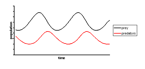
solutions which do not have a simple expression in terms of the usual trigonometric functions. However, a linearization
of the equations yields a solution similar to simple harmonic motion
with the population of predators following that of prey by 90°.
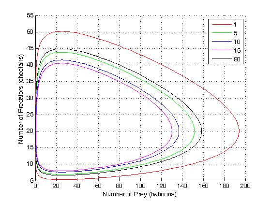
One can also plot a solution which corresponds to the oscillatory nature of the population of the two species. This solution is in a state of dynamic equilibrium. At any given time in this phase plane
, the system is in a limit cycle and lies somewhere on the inside of these elliptical solutions. There is no particular requirement on the system to begin within a limit cycle and thus in a stable solution, however, it will always reach one eventually.
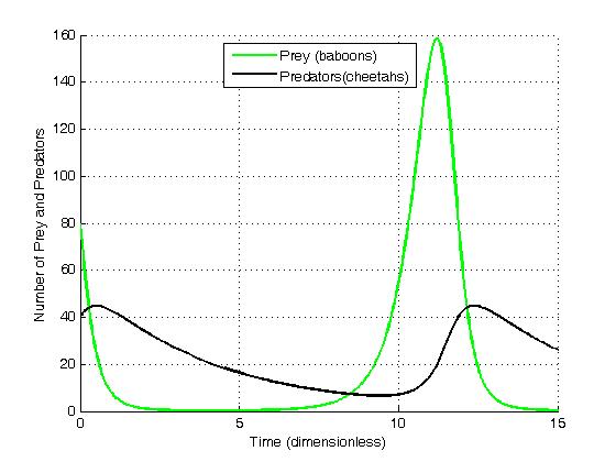
These graphs clearly illustrate a serious problem with this as a biological model: in each cycle, the baboon population is reduced to extremely low numbers yet recovers (while the cheetah population remains sizeable at the lowest baboon density). Given chance fluctuations, discrete numbers of individuals, and the family structure and lifecycle of baboons, the baboons actually go extinct and by consequence the cheetahs as well. This modelling problem has been called the "atto-fox problem", an atto-fox being an imaginary 10−18 of a fox, in relation to rabies modelling in the UK.


When solved for x and y the above system of equations yields

and

Hence, there are two equilibria.
The first solution effectively represents the extinction of both species. If both populations are at 0, then they will continue to be so indefinitely. The second solution represents a fixed point at which both populations sustain their current, non-zero numbers, and, in the simplified model, do so indefinitely. The levels of population at which this equilibrium is achieved depend on the chosen values of the parameters, α, β, γ, and δ.
using partial derivative
s, while the other fixed point requires a slightly more sophisticated method.
The Jacobian matrix of the predator-prey model is


The eigenvalues of this matrix are

In the model α and γ are always greater than zero, and as such the sign of the eigenvalues above will always differ. Hence the fixed point at the origin is a saddle point
.
The stability of this fixed point is of importance. If it were stable, non-zero populations might be attracted towards it, and as such the dynamics of the system might lead towards the extinction of both species for many cases of initial population levels. However, as the fixed point at the origin is a saddle point, and hence unstable, we find that the extinction of both species is difficult in the model. (In fact, this can only occur if the prey are artificially completely eradicated, causing the predators to die of starvation. If the predators are eradicated, the prey population grows without bound in this simple model).

The eigenvalues of this matrix are

As the eigenvalues are both purely imaginary, this fixed point is not hyperbolic
, so no conclusions can be drawn from the linear analysis. However, the system admits a constant of motion

and the level curves, where K = const, are closed trajectories surrounding the fixed point.
Consequently, the levels of the predator and prey populations cycle, and oscillate around this fixed point.
The largest value of the constant K can be obtained by solving the optimization problem
The maximal value of K is attained at the stationary point and it is given by

where e is Euler's Number
.
Differential equation
A differential equation is a mathematical equation for an unknown function of one or several variables that relates the values of the function itself and its derivatives of various orders...
s frequently used to describe the dynamics
Dynamical system
A dynamical system is a concept in mathematics where a fixed rule describes the time dependence of a point in a geometrical space. Examples include the mathematical models that describe the swinging of a clock pendulum, the flow of water in a pipe, and the number of fish each springtime in a...
of biological systems
Systems biology
Systems biology is a term used to describe a number of trends in bioscience research, and a movement which draws on those trends. Proponents describe systems biology as a biology-based inter-disciplinary study field that focuses on complex interactions in biological systems, claiming that it uses...
in which two species interact, one a predator and one its prey. They evolve in time according to the pair of equations:
where,
- y is the number of some predatorPredationIn ecology, predation describes a biological interaction where a predator feeds on its prey . Predators may or may not kill their prey prior to feeding on them, but the act of predation always results in the death of its prey and the eventual absorption of the prey's tissue through consumption...
(for example, foxesFoxFox is a common name for many species of omnivorous mammals belonging to the Canidae family. Foxes are small to medium-sized canids , characterized by possessing a long narrow snout, and a bushy tail .Members of about 37 species are referred to as foxes, of which only 12 species actually belong to...
); - x is the number of its prey (for example, rabbitRabbitRabbits are small mammals in the family Leporidae of the order Lagomorpha, found in several parts of the world...
s);  and
and  represent the growth of the two populations against time;
- t represents the time; and
- α, β, γ and δ are parameterParameterParameter from Ancient Greek παρά also “para” meaning “beside, subsidiary” and μέτρον also “metron” meaning “measure”, can be interpreted in mathematics, logic, linguistics, environmental science and other disciplines....
s representing the interaction of the two speciesSpeciesIn biology, a species is one of the basic units of biological classification and a taxonomic rank. A species is often defined as a group of organisms capable of interbreeding and producing fertile offspring. While in many cases this definition is adequate, more precise or differing measures are...
.
The Lotka–Volterra system of equations is an example of a Kolmogorov model, which is a more general framework that can model the dynamics of ecological systems with predator-prey interactions, competition, disease, and mutualism.
History
The Lotka–Volterra predator–prey modelMathematical model
A mathematical model is a description of a system using mathematical concepts and language. The process of developing a mathematical model is termed mathematical modeling. Mathematical models are used not only in the natural sciences and engineering disciplines A mathematical model is a...
was initially proposed by Alfred J. Lotka
Alfred J. Lotka
Alfred James Lotka was a US mathematician, physical chemist, and statistician, famous for his work in population dynamics and energetics. An American biophysicist best known for his proposal of the predator-prey model, developed simultaneously but independently of Vito Volterra...
“in the theory of autocatalytic chemical reactions” in 1910. This was effectively the logistic equation, which was originally derived by Pierre François Verhulst
Pierre François Verhulst
Pierre François Verhulst was a mathematician and a doctor in number theory from the University of Ghent in 1825...
. In 1920 Lotka extended, via Kolmogorov (see above), the model to "organic systems" using a plant species and a herbivorous animal species as an example and in 1925 he utilised the equations to analyse predator-prey interactions in his book on biomathematics arriving at the equations that we know today. Vito Volterra
Vito Volterra
Vito Volterra was an Italian mathematician and physicist, known for his contributions to mathematical biology and integral equations....
, who made a statistical analysis of fish catches in the Adriatic independently investigated the equations in 1926.
C.S. Holling extended this model yet again, in two 1959 papers, in which he proposed the idea of functional response
Functional response
A functional response in ecology is the intake rate of a consumer as a function of food density. It is associated with the numerical response, which is the reproduction rate of a consumer as a function of food density. Following C. S...
. Both the Lotka-Volterra model and Holling's extensions have been used to model the moose and wolf populations in Isle Royale National Park
Isle Royale National Park
Isle Royale National Park is a U.S. National Park in the state of Michigan. Isle Royale, the largest island in Lake Superior, is over 45 miles in length and 9 miles wide at its widest point. The park is made of Isle Royale itself and approximately 400 smaller islands, along with any submerged...
, which with over 50 published papers is one of the best studied predator-prey relationships.
In economics
The Lotka–Volterra equations have a long history of use in economic theory; their initial application is commonly credited to Richard GoodwinRichard M. Goodwin
Richard M. Goodwin was an American mathematician and economist. He was born in Indiana.Goodwin received his BA and PhD at Harvard, and he taught there from 1942 until 1950. He taught at the University of Cambridge until 1979 and the University of Siena until 1984.Goodwin worked on the interaction...
in 1965 or 1967. In economics, links are between many if not all industries; a proposed way to model the dynamics of various industries has been by introducing trophic functions between various sectors, and ignoring smaller sectors by considering the interactions of only two industrial sectors.
Physical meanings of the equations
The Lotka-Volterra model makes a number of assumptions about the environment and evolution of the predator and prey populations:- The prey population finds ample food at all times.
- The food supply of the predator population depends entirely on the prey populations.
- The rate of change of population is proportional to its size.
- During the process, the environment does not change in favour of one species and the genetic adaptation is sufficiently slow.
As differential equations are used, the solution is deterministic
Determinism
Determinism is the general philosophical thesis that states that for everything that happens there are conditions such that, given them, nothing else could happen. There are many versions of this thesis. Each of them rests upon various alleged connections, and interdependencies of things and...
and continuous
Continuous function
In mathematics, a continuous function is a function for which, intuitively, "small" changes in the input result in "small" changes in the output. Otherwise, a function is said to be "discontinuous". A continuous function with a continuous inverse function is called "bicontinuous".Continuity of...
. This, in turn, implies that the generations of both the predator and prey are continually overlapping.
Prey
When multiplied out, the prey equation becomes:The prey are assumed to have an unlimited food supply, and to reproduce exponentially unless subject to predation; this exponential growth
Exponential growth
Exponential growth occurs when the growth rate of a mathematical function is proportional to the function's current value...
is represented in the equation above by the term αx. The rate of predation upon the prey is assumed to be proportional to the rate at which the predators and the prey meet; this is represented above by βxy. If either x or y is zero then there can be no predation.
With these two terms the equation above can be interpreted as: the change in the prey's numbers is given by its own growth minus the rate at which it is preyed upon.
Predators
The predator equation becomes:In this equation, δxy represents the growth of the predator population. (Note the similarity to the predation rate; however, a different constant is used as the rate at which the predator population grows is not necessarily equal to the rate at which it consumes the prey). γy represents the loss rate of the predators due to either natural death or emigration; it leads to an exponential decay in the absence of prey.
Hence the equation expresses the change in the predator population as growth fueled by the food supply, minus natural death.
Solutions to the equations
The equations have periodicPeriodic function
In mathematics, a periodic function is a function that repeats its values in regular intervals or periods. The most important examples are the trigonometric functions, which repeat over intervals of length 2π radians. Periodic functions are used throughout science to describe oscillations,...
solutions which do not have a simple expression in terms of the usual trigonometric functions. However, a linearization
Linearization
In mathematics and its applications, linearization refers to finding the linear approximation to a function at a given point. In the study of dynamical systems, linearization is a method for assessing the local stability of an equilibrium point of a system of nonlinear differential equations or...
of the equations yields a solution similar to simple harmonic motion
Simple harmonic motion
Simple harmonic motion can serve as a mathematical model of a variety of motions, such as the oscillation of a spring. Additionally, other phenomena can be approximated by simple harmonic motion, including the motion of a simple pendulum and molecular vibration....
with the population of predators following that of prey by 90°.
An example problem
Suppose there are two species of animals, a baboon (prey) and a cheetah (predator). If the initial conditions are 80 baboons and 40 cheetahs, one can plot the progression of the two species over time. The choice of time interval is arbitrary.One can also plot a solution which corresponds to the oscillatory nature of the population of the two species. This solution is in a state of dynamic equilibrium. At any given time in this phase plane
Phase plane
A phase plane is a visual display of certain characteristics of certain kinds of differential equations; it is a 2-dimensional version of the general n-dimensional phase space....
, the system is in a limit cycle and lies somewhere on the inside of these elliptical solutions. There is no particular requirement on the system to begin within a limit cycle and thus in a stable solution, however, it will always reach one eventually.
These graphs clearly illustrate a serious problem with this as a biological model: in each cycle, the baboon population is reduced to extremely low numbers yet recovers (while the cheetah population remains sizeable at the lowest baboon density). Given chance fluctuations, discrete numbers of individuals, and the family structure and lifecycle of baboons, the baboons actually go extinct and by consequence the cheetahs as well. This modelling problem has been called the "atto-fox problem", an atto-
Dynamics of the system
In the model system, the predators thrive when there are plentiful prey but, ultimately, outstrip their food supply and decline. As the predator population is low the prey population will increase again. These dynamics continue in a cycle of growth and decline.Population equilibrium
Population equilibrium occurs in the model when neither of the population levels is changing, i.e. when both of the derivatives are equal to 0.When solved for x and y the above system of equations yields
and
Hence, there are two equilibria.
The first solution effectively represents the extinction of both species. If both populations are at 0, then they will continue to be so indefinitely. The second solution represents a fixed point at which both populations sustain their current, non-zero numbers, and, in the simplified model, do so indefinitely. The levels of population at which this equilibrium is achieved depend on the chosen values of the parameters, α, β, γ, and δ.
Stability of the fixed points
The stability of the fixed point at the origin can be determined by performing a linearizationLinearization
In mathematics and its applications, linearization refers to finding the linear approximation to a function at a given point. In the study of dynamical systems, linearization is a method for assessing the local stability of an equilibrium point of a system of nonlinear differential equations or...
using partial derivative
Partial derivative
In mathematics, a partial derivative of a function of several variables is its derivative with respect to one of those variables, with the others held constant...
s, while the other fixed point requires a slightly more sophisticated method.
The Jacobian matrix of the predator-prey model is
First fixed point
When evaluated at the steady state of (0, 0) the Jacobian matrix J becomesThe eigenvalues of this matrix are
In the model α and γ are always greater than zero, and as such the sign of the eigenvalues above will always differ. Hence the fixed point at the origin is a saddle point
Saddle point
In mathematics, a saddle point is a point in the domain of a function that is a stationary point but not a local extremum. The name derives from the fact that in two dimensions the surface resembles a saddle that curves up in one direction, and curves down in a different direction...
.
The stability of this fixed point is of importance. If it were stable, non-zero populations might be attracted towards it, and as such the dynamics of the system might lead towards the extinction of both species for many cases of initial population levels. However, as the fixed point at the origin is a saddle point, and hence unstable, we find that the extinction of both species is difficult in the model. (In fact, this can only occur if the prey are artificially completely eradicated, causing the predators to die of starvation. If the predators are eradicated, the prey population grows without bound in this simple model).
Second fixed point
Evaluating J at the second fixed point we getThe eigenvalues of this matrix are
As the eigenvalues are both purely imaginary, this fixed point is not hyperbolic
Hyperbolic equilibrium point
In the study of dynamical systems, a hyperbolic equilibrium point or hyperbolic fixed point is a fixed point that does not have any center manifolds. Near a hyperbolic point the orbits of a two-dimensional, non-dissipative system resemble hyperbolas. This fails to hold in general...
, so no conclusions can be drawn from the linear analysis. However, the system admits a constant of motion
Constant of motion
In mechanics, a constant of motion is a quantity that is conserved throughout the motion, imposing in effect a constraint on the motion. However, it is a mathematical constraint, the natural consequence of the equations of motion, rather than a physical constraint...
and the level curves, where K = const, are closed trajectories surrounding the fixed point.
Consequently, the levels of the predator and prey populations cycle, and oscillate around this fixed point.
The largest value of the constant K can be obtained by solving the optimization problem
The maximal value of K is attained at the stationary point
and it is given bywhere e is Euler's Number
E (mathematical constant)
The mathematical constant ' is the unique real number such that the value of the derivative of the function at the point is equal to 1. The function so defined is called the exponential function, and its inverse is the natural logarithm, or logarithm to base...
.
See also
- Competitive Lotka–Volterra equations
- Generalized Lotka–Volterra equationGeneralized Lotka–Volterra equationThe generalized Lotka–Volterra equations are a set of equations which are more general than either the competitive or predator-prey examples of Lotka–Volterra types. They can be used to model direct competition and trophic relationships between an arbitrary number of species. Their...
- Mutualism and the Lotka–Volterra equation
- Community matrixCommunity matrixIn mathematical biology, the community matrix is the linearization of the Lotka–Volterra equation at an equilibrium point. The eigenvalues of the community matrix determine the stability of the equilibrium point....
- Population dynamicsPopulation dynamicsPopulation dynamics is the branch of life sciences that studies short-term and long-term changes in the size and age composition of populations, and the biological and environmental processes influencing those changes...
- Population dynamics of fisheriesPopulation dynamics of fisheriesA fishery is an area with an associated fish or aquatic population which is harvested for its commercial or recreational value. Fisheries can be wild or farmed. Population dynamics describes the ways in which a given population grows and shrinks over time, as controlled by birth, death, and...
- Nicholson–Bailey model
External links
- Lotka–Volterra Predator-Prey Model by Elmer G. Wiens
- Lotka-Volterra Model
- NANIA Lotka-Volterra applet
- Lotka Algorithmic Simulation Similar program, in Javascript (requires an HTML5 browser).
- From the Wolfram Demonstrations ProjectWolfram Demonstrations ProjectThe Wolfram Demonstrations Project is hosted by Wolfram Research, whose stated goal is to bring computational exploration to the widest possible audience. It consists of an organized, open-source collection of small interactive programs called Demonstrations, which are meant to visually and...
— requires CDF player (free):