Linear canonical transformation - AbsoluteAstronomy.com

Hamiltonian mechanics

Hamiltonian mechanics is a reformulation of classical mechanics that was introduced in 1833 by Irish mathematician William Rowan Hamilton.It arose from Lagrangian mechanics, a previous reformulation of classical mechanics introduced by Joseph Louis Lagrange in 1788, but can be formulated without...

, the linear canonical transformation (LCT) is a family of integral transforms that generalizes many classical transforms. It has 4 parameters and 1 constraint, so it is a 3-dimensional family, and can be visualized as the action of the special linear group

Special linear group

In mathematics, the special linear group of degree n over a field F is the set of n×n matrices with determinant 1, with the group operations of ordinary matrix multiplication and matrix inversion....

SL₂(R) on the time–frequency plane (domain).

The LCT generalizes the Fourier

Fourier transform

In mathematics, Fourier analysis is a subject area which grew from the study of Fourier series. The subject began with the study of the way general functions may be represented by sums of simpler trigonometric functions...

, fractional Fourier

Fractional Fourier transform

In mathematics, in the area of harmonic analysis, the fractional Fourier transform is a linear transformation generalizing the Fourier transform. It can be thought of as the Fourier transform to the n-th power where n need not be an integer — thus, it can transform a function to an...

, Laplace, Gauss–Weierstrass

Weierstrass transform

In mathematics, the Weierstrass transform of a function f : R → R, named after Karl Weierstrass, is the function F defined by...

, Bargmann and the Fresnel transforms as particular cases. The name "linear canonical transformation" is from canonical transformation

Canonical transformation

In Hamiltonian mechanics, a canonical transformation is a change of canonical coordinates → that preserves the form of Hamilton's equations , although it...

, a map that preserves the symplectic structure, as SL₂(R) can also be interpreted as the symplectic group

Symplectic group

In mathematics, the name symplectic group can refer to two different, but closely related, types of mathematical groups, denoted Sp and Sp. The latter is sometimes called the compact symplectic group to distinguish it from the former. Many authors prefer slightly different notations, usually...

Sp₂, and thus LCTs are the linear maps of the time–frequency domain which preserve the symplectic form.

Definition

The LCT can be represented in several ways; most easily, it can be viewed as a 2×2 matrix with determinant 1, i.e., an element of the special linear group

Special linear group

SL₂(R). Taking a matrix

with ad − bc = 1, the corresponding integral transform is:

	when b ≠ 0,
	when b = 0.

Special cases

Many classical transforms are special cases of the linear canonical transform:

The Fourier transform
Fourier transform
In mathematics, Fourier analysis is a subject area which grew from the study of Fourier series. The subject began with the study of the way general functions may be represented by sums of simpler trigonometric functions...

corresponds to rotation by 90°, represented by the matrix:

The fractional Fourier transform
Fractional Fourier transform
In mathematics, in the area of harmonic analysis, the fractional Fourier transform is a linear transformation generalizing the Fourier transform. It can be thought of as the Fourier transform to the n-th power where n need not be an integer — thus, it can transform a function to an...

corresponds to rotation by an arbitrary angle; they are the elliptic elements of SL₂(R), represented by the matrices:

The Fresnel transform corresponds to shearing, and are a family of parabolic elements, represented by the matrices:

where z is distance and λ is wave length.

Composition

Composition of LCTs corresponds to multiplication of the corresponding matrices; this is also known as the "additivity property of the WDF

Wigner distribution function

The Wigner distribution function was first proposed to account for quantum corrections to classical statistical mechanics in 1932 by Eugene Wigner, cf. Wigner quasi-probability distribution....

".

In detail, if the LCT is denoted by O_F^(a,b,c,d), i.e.

then

where

In optics and quantum mechanics

Paraxial optical systems implemented entirely with thin lens

Thin lens

es and propagation through free space and/or graded index (GRIN) media, are quadratic phase systems (QPS); these were known before Moshinsky and Quesne (1974) called attention to their significance in connection with canonical transformations in quantum mechanics. The effect of any arbitrary QPS on an input wavefield can be described using the linear canonical transform, a particular case of which was developed by Segal (1963) and Bargmann (1961) in order to formalize Fok's (1928) boson calculus.

Applications

Canonical transforms provide a fine tool for the analysis of a class of differential equations. These include diffusion

Diffusion

Molecular diffusion, often called simply diffusion, is the thermal motion of all particles at temperatures above absolute zero. The rate of this movement is a function of temperature, viscosity of the fluid and the size of the particles...

, the Schrödinger free particle

Free particle

In physics, a free particle is a particle that, in some sense, is not bound. In classical physics, this means the particle is present in a "field-free" space.-Classical Free Particle:The classical free particle is characterized simply by a fixed velocity...

, the linear potential (free-fall), and the attractive and repulsive oscillator equations. It also includes a few others such as the Fokker–Planck equation. Although this class is far from universal, the ease with which solutions and properties are found makes canonical transforms an attractive tool for problems such as these.

Wave propagation through air, a lens, and between satellite dishes are discussed here. All of the computations can be reduced to 2×2 matrix algebra. This is the spirit of LCT.

Electromagnetic wave propagation

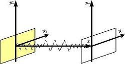
Assuming the system looks like as depicted in the figure, the wave travels from plane x_i, y_i to the plane of x and y.
The Fresnel transform is used to describe electromagnetic wave propagation in air:

with

k = 2 π / λ	: wave number;
λ	: wavelength Wavelength In physics, the wavelength of a sinusoidal wave is the spatial period of the wave—the distance over which the wave's shape repeats.It is usually determined by considering the distance between consecutive corresponding points of the same phase, such as crests, troughs, or zero crossings, and is a... ;
z	: distance of propagation;
j	: imaginary unit.

This is equivalent to LCT (shearing), when

When the travel distance (z) is larger, the shearing effect is larger.

Spherical lens

With the lens as depicted in the figure, and the refractive index denoted as n, the result is: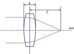

with f the focal length and Δ the thickness of the lens.

The distortion passing through the lens is similar to LCT, when

This is also a shearing effect: when the focal length is smaller, the shearing effect is larger.

Satellite dish

The satellite dish can be described as a LCT, with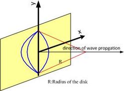

This is very similar to lens, except focal length is replaced by the radius of the dish. Therefore, if the radius is larger, the shearing effect is larger.

Example

The system considered is depicted in the figure to the right: two dishes – one being the emitter and the other one the receiver – and a signal travelling between them over a distance D.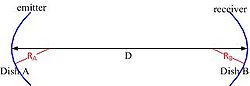
First, for dish A (emitter), the LCT matrix looks like this:

Then, for dish B (receiver), the LCT matrix similarly becomes:

Last, for the propagation of the signal in air, the LCT matrix is:

Putting all three components together, the LCT of the system is: