Gradient descent is a first-order optimization algorithm
Algorithm
In mathematics and computer science, an algorithm is an effective method expressed as a finite list of well-defined instructions for calculating a function. Algorithms are used for calculation, data processing, and automated reasoning...
. To find a local minimum of a function using gradient descent, one takes steps proportional to the negative of the gradient
Gradient
In vector calculus, the gradient of a scalar field is a vector field that points in the direction of the greatest rate of increase of the scalar field, and whose magnitude is the greatest rate of change....
(or of the approximate gradient) of the function at the current point. If instead one takes steps proportional to the positive of the gradient
Gradient
In vector calculus, the gradient of a scalar field is a vector field that points in the direction of the greatest rate of increase of the scalar field, and whose magnitude is the greatest rate of change....
, one approaches a local maximum of that function; the procedure is then known as gradient ascent.
Gradient descent is also known as steepest descent, or the method of steepest descent. When known as the latter, gradient descent should not be confused with the method of steepest descent for approximating integrals.
Description
Gradient descent is based on the observation that if the multivariable function is defined and differentiable
Differentiable function
In calculus , a differentiable function is a function whose derivative exists at each point in its domain. The graph of a differentiable function must have a non-vertical tangent line at each point in its domain...
in a neighborhood of a point , then decreases fastest if one goes from in the direction of the negative gradient of at , . It follows that, if
for a small enough number, then . With this observation in mind, one starts with a guess for a local minimum of , and considers the sequence such that
We have
so hopefully the sequence converges to the desired local minimum. Note that the value of the step size is allowed to change at every iteration.
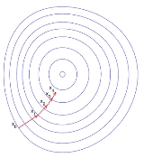
This process is illustrated in the picture to the right. Here is assumed to be defined on the plane, and that its graph has a bowl
Bowl (vessel)
A bowl is a common open-top container used in many cultures to serve food, and is also used for drinking and storing other items. They are typically small and shallow, although some, such as punch bowls and salad bowls, are larger and often intended to serve many people.Bowls have existed for...
A contour line of a function of two variables is a curve along which the function has a constant value. In cartography, a contour line joins points of equal elevation above a given level, such as mean sea level...
s, that is, the regions on which the value of is constant. A red arrow originating at a point shows the direction of the negative gradient at that point. Note that the (negative) gradient at a point is orthogonal to the contour line going through that point. We see that gradient descent leads us to the bottom of the bowl, that is, to the point where the value of the function is minimal.
Examples
Gradient descent has problems with pathological functions such as the Rosenbrock function
Rosenbrock function
In mathematical optimization, the Rosenbrock function is a non-convex function used as a performance test problem for optimization algorithms introduced by Howard H. Rosenbrock in 1960. It is also known as Rosenbrock's valley or Rosenbrock's banana function.The global minimum is inside a long,...
shown here.
The Rosenbrock function has a narrow curved valley which contains the minimum. The bottom of the valley is very flat. Because of the curved flat valley the optimization is zig-zagging slowly with small stepsizes towards the minimum.
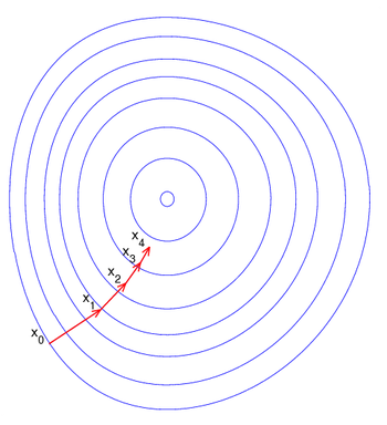
The "Zig-Zagging" nature of the method is also evident below, where the gradient ascent method is applied to .
>
Limitations
For some of the above examples, gradient descent is relatively slow close to the minimum: Technically, its asymptotic rate of convergence is inferior to other methods. For poorly conditioned convex problems, gradient descent increasingly 'zigzags' as the gradients point nearly orthogonally to the shortest direction to a minimum point. For more details, see Comments below:
For non-differentiable functions, gradient methods are ill-defined. For locally Lipschitz
Lipschitz continuity
In mathematical analysis, Lipschitz continuity, named after Rudolf Lipschitz, is a strong form of uniform continuity for functions. Intuitively, a Lipschitz continuous function is limited in how fast it can change: for every pair of points on the graph of this function, the absolute value of the...
Subgradient methods are iterative methods for solving convex minimization problems. Originally developed by Naum Z. Shor and others in the 1960s and 1970s, subgradient methods are convergent when applied even to a non-differentiable objective function...
are well-defined. Non-descent methods, like subgradient projection methods, may also be used.
Solution of a linear system
Gradient descent can be used to solve a system of linear equations, reformulated as a quadratic minimization problem, e.g., using linear least squares
Linear least squares
In statistics and mathematics, linear least squares is an approach to fitting a mathematical or statistical model to data in cases where the idealized value provided by the model for any data point is expressed linearly in terms of the unknown parameters of the model...
. Solution of
in the sense of linear least squares is defined as minimizing the function
In traditional linear least squares for real and the Euclidean norm is used, in which case
In the case that is real, square, symmetric and positive definite, a different popular choice of the norm is
which produces a different equation with a better condition number
Condition number
In the field of numerical analysis, the condition number of a function with respect to an argument measures the asymptotically worst case of how much the function can change in proportion to small changes in the argument...
:
In either case, the line search minimization, finding the locally optimal step size on every iteration, can be performed analytically, and explicit formulas for the locally optimal are known. https://hpcrd.lbl.gov/~meza/papers/Steepest%20Descent.pdf
Solution of a non-linear system
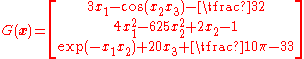
Gradient descent can also be used to solve a system of nonlinear equations. Below is an example that shows how to use the gradient descent to solve for three unknown variables, x1, x2, and x3. This example shows one iteration of the gradient descent.
Consider a nonlinear system of equations:
suppose we have the function
where
and the objective function
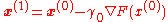
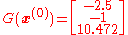
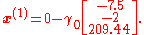
With initial guess
We know that
where
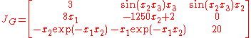
The Jacobian matrix
Then evaluating these terms at
and
So that
and
Now a suitable must be found such that . This can be done with any of a variety of line search algorithms. One might also simply guess which gives
evaluating at this value,
The decrease from to the next step's value of is a sizable decrease in the objective function. Further steps would reduce its value until a solution to the system was found.
Comments
Gradient descent works in spaces of any number of dimensions, even in infinite-dimensional ones. In the latter case the search space is typically a function space
Function space
In mathematics, a function space is a set of functions of a given kind from a set X to a set Y. It is called a space because in many applications it is a topological space, a vector space, or both.-Examples:...
In mathematics, the Gâteaux differential or Gâteaux derivative is a generalization of the concept of directional derivative in differential calculus. Named after René Gâteaux, a French mathematician who died young in World War I, it is defined for functions between locally convex topological vector...
of the functional to be minimized to determine the descent direction.
The gradient descent can take many iterations to compute a local minimum with a required accuracy, if the curvature
Curvature
In mathematics, curvature refers to any of a number of loosely related concepts in different areas of geometry. Intuitively, curvature is the amount by which a geometric object deviates from being flat, or straight in the case of a line, but this is defined in different ways depending on the context...
in different directions is very different for the given function. For such functions, preconditioning, which changes the geometry of the space to shape the function level sets like concentric circles, cures the slow convergence. Constructing and applying preconditioning can be computationally expensive, however.
The gradient descent can be combined with a line search, finding the locally optimal step size on every iteration. Performing the line search can be time-consuming. Conversely, using a fixed small can yield poor convergence.
In mathematics, Newton's method is an iterative method for finding roots of equations. More generally, Newton's method is used to find critical points of differentiable functions, which are the zeros of the derivative function.-Method:...
In mathematics, the Hessian matrix is the square matrix of second-order partial derivatives of a function; that is, it describes the local curvature of a function of many variables. The Hessian matrix was developed in the 19th century by the German mathematician Ludwig Otto Hesse and later named...
using conjugate gradient techniques can be better alternatives. Generally, such methods converge in fewer iterations, but the cost of each iteration is higher. An example is the BFGS method
BFGS method
In numerical optimization, the Broyden–Fletcher–Goldfarb–Shanno method is a method for solving nonlinear optimization problems ....
which consists in calculating on every step a matrix by which the gradient vector is multiplied to go into a "better" direction, combined with a more sophisticated line search algorithm, to find the "best" value of For extremely large problems, where the computer memory issues dominate, a limited-memory method such as L-BFGS should be used instead of BFGS or the steepest descent.
Gradient descent can be viewed as Euler's method for solving ordinary differential equations of a gradient flow.
A computational example
The gradient descent algorithm is applied to find a local minimum of the function f(x)=x4−3x3+2, with derivative f'(x)=4x3−9x2. Here is an implementation in the Python programming language.
From calculation, we expect that the local minimum occurs at x=9/4
The above piece of code has to be modified with regard to step size according to the system at hand and convergence can be made faster by using an adaptive step size. In the above case the step size is not adaptive. It stays at 0.01 in all the directions which can sometimes cause the method to fail by diverging from the minimum.
Stochastic gradient descent is an optimization method for minimizing an objective function that is written as a sum of differentiable functions.- Background :...
Rprop, short for resilient backpropagation, is a learning heuristic for supervised learning in feedforward artificial neural networks. This is a first-order optimization algorithm...
In mathematics, Newton's method is an iterative method for finding roots of equations. More generally, Newton's method is used to find critical points of differentiable functions, which are the zeros of the derivative function.-Method:...
The delta rule is a gradient descent learning rule for updating the weights of the artificial neurons in a single-layer perceptron. It is a special case of the more general backpropagation algorithm...
In the unconstrained minimization problem, the Wolfe conditions are a set of inequalities for performing inexact line search, especially in quasi-Newton methods.In these methods the idea is to find\min_x f...
Preconditioning
The source of this article is wikipedia, the free encyclopedia. The text of this article is licensed under the GFDL.

 Gradient descent is based on the observation that if the multivariable function
  is defined and differentiable
 , then
  decreases fastest if one goes from
  in the direction of the negative gradient of
  at
at  ,
,  . It follows that, if
 a small enough number, then
  . With this observation in mind, one starts with a guess
  for a local minimum of
  , and considers the sequence
 such that

 converges to the desired local minimum. Note that the value of the step size
  is allowed to change at every iteration.
 is assumed to be defined on the plane, and that its graph has a bowl
 is constant. A red arrow originating at a point shows the direction of the negative gradient at that point. Note that the (negative) gradient at a point is orthogonal to the contour line going through that point. We see that gradient descent leads us to the bottom of the bowl, that is, to the point where the value of the function
  is minimal.
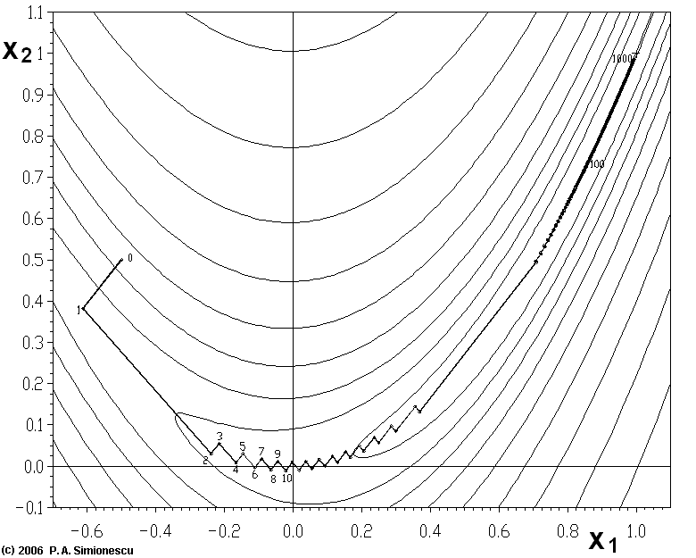 The "Zig-Zagging" nature of the method is also evident below, where the gradient ascent method is applied to
  .
..png)
.png) >
>


 and
and  the Euclidean norm is used, in which case
 is real, square, symmetric and positive definite, a different popular choice of the norm is

 on every iteration, can be performed analytically, and explicit formulas for the locally optimal
  are known. https://hpcrd.lbl.gov/~meza/papers/Steepest%20Descent.pdf


 must be found such that
 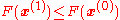 . This can be done with any of a variety of line search algorithms. One might also simply guess
  which gives
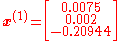

 to the next step's value of
 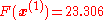 is a sizable decrease in the objective function. Further steps would reduce its value until a solution to the system was found.
 on every iteration. Performing the line search can be time-consuming. Conversely, using a fixed small
  can yield poor convergence.
 For extremely large problems, where the computer memory issues dominate, a limited-memory method such as L-BFGS should be used instead of BFGS or the steepest descent.
 of a gradient flow.
