
Gauss-Newton algorithm
Encyclopedia
The Gauss–Newton algorithm is a method used to solve non-linear least squares
problems. It can be seen as a modification of Newton's method
for finding a minimum
of a function
. Unlike Newton's method, the Gauss–Newton algorithm can only be used to minimize a sum of squared function values, but it has the advantage that second derivatives, which can be challenging to compute, are not required.
Non-linear least squares problems arise for instance in non-linear regression, where parameters in a model are sought such that the model is in good agreement with available observations.
The method is named after the mathematicians Carl Friedrich Gauss
and Isaac Newton
.

Starting with an initial guess for the minimum, the method proceeds by the iterations

where Δ is a small step. We then have .
.
If we define the Jacobian matrix ,
,
we can replace with
with 
and the Hessian matrix
in the right can be approximated by (assuming small residual), giving:
 .
.
We then take the derivative with respect to and set it equal to zero to find a solution:
 .
.
This can be rearranged to give the normal equations which can be solved for Δ:

In data fitting, where the goal is to find the parameters β such that a given model function y = f(x, β) fits best some data points (xi, yi), the functions ri are the residuals
Then, the increment can be expressed in terms of the Jacobian of the
function f, as
 In this example, the Gauss–Newton algorithm will be used to fit a model to some data by minimizing the sum of squares of errors between the data and model's predictions.
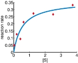
In a biology experiment studying the relation between substrate concentration [S] and reaction rate in an enzyme-mediated reaction, the data in the following table were obtained.
It is desired to find a curve (model function) of the form
that fits best the data in the least squares sense, with the parameters and
and  to be determined.
Denote by and
and  the value of
  and the rate from the table,
  Let
Let  and
and  We will find
  and
and  such that the sum of squares of the residuals
is minimized.
The Jacobian of the vector of residuals
  in respect to the unknowns
  is an
is an  matrix with the
  -th row having the entries
Starting with the initial estimates of =0.9 and
  =0.2, after five iterations of the Gauss–Newton algorithm the optimal values
  and
and  are obtained. The sum of squares of residuals decreased from the initial value of 1.445 to 0.00784 after the fifth iteration. The plot in the figure on the right shows the curve determined by the model for the optimal parameters versus the observed data.
of S. However, convergence is not guaranteed, not even local convergence
as in Newton's method
.
The rate of convergence of the Gauss–Newton algorithm can approach quadratic
. The algorithm may converge slowly or not at all if the initial guess is far from the minimum or the matrix is ill-conditioned. For example, consider the problem with
  equations and
  variable, given by
The optimum is at . If
. If  then the problem is in fact linear and the method finds the optimum in one iteration. If |λ| < 1 then the method converges linearly and the error decreases asymptotically with a factor |λ| at every iteration. However, if |λ| > 1, then the method does not even converge locally.
for function optimization via an approximation. As a consequence, the rate of convergence of the Gauss–Newton algorithm is at most quadratic.
The recurrence relation for Newton's method for minimizing a function S of parameters, β, is
where g denotes the gradient vector
of S and H denotes the Hessian matrix
of S.
Since , the gradient is given by
Elements of the Hessian are calculated by differentiating the gradient elements, , with respect to
The Gauss–Newton method is obtained by ignoring the second-order derivative terms (the second term in this expression). That is, the Hessian is approximated by
where are entries of the Jacobian Jr. The gradient and the approximate Hessian can be written in matrix notation as

These expressions are substituted into the recurrence relation above to obtain the operational equations

Convergence of the Gauss–Newton method is not guaranteed in all instances. The approximation
that needs to hold to be able to ignore the second-order derivative terms may be valid in two cases, for which convergence is to be expected.
 is a stationary point, it holds that
  for all sufficiently small
  . Thus, if divergence occurs, one solution is to employ a fraction,
  , of the increment vector, Δ in the updating formula
 .
.
In other words, the increment vector is too long, but it points in "downhill", so going just a part of the way will decrease the objective function S. An optimal value for can be found by using a line search algorithm, that is, the magnitude of
  is determined by finding the value that minimizes S, usually using a direct search method in the interval
  .
.
In cases where the direction of the shift vector is such that the optimal fraction, , is close to zero, an alternative method for handling divergence is the use of the Levenberg–Marquardt algorithm, also known as the "trust region method". The normal equations are modified in such a way that the increment vector is rotated towards the direction of steepest descent,
  ,
,
where D is a positive diagonal matrix. Note that when D is the identity matrix and , then
  , therefore the direction
of Δ approaches the direction of the gradient .
.
The so-called Marquardt parameter, , may also be optimized by a line search, but this is inefficient as the shift vector must be re-calculated every time
  is changed. A more efficient strategy is this. When divergence occurs increase the Marquardt parameter until there is a decrease in S. Then, retain the value from one iteration to the next, but decrease it if possible until a cut-off value is reached when the Marquardt parameter can be set to zero; the minimization of S then becomes a standard Gauss–Newton minimization.
, such as that due to Davidon, Fletcher and Powell or Broyden–Fletcher–Goldfarb–Shanno (BFGS) an estimate of the full Hessian, , is built up numerically using first derivatives
  only so that after n refinement cycles the method closely approximates to Newton's method in performance. Note that quasi-Newton methods can minimize general real-valued functions, whereas Gauss-Newton, Levenberg-Marquardt, etc. fits only to nonlinear least-squares problems.
Another method for solving minimization problems using only first derivatives is gradient descent
. However, this method does not take into account the second derivatives even approximately. Consequently, it is highly inefficient for many functions, especially if the parameters have strong interactions.
Non-linear least squares
Non-linear least squares is the form of least squares analysis which is used to fit a set of m observations with a model that is non-linear in n unknown parameters . It is used in some forms of non-linear regression. The basis of the method is to approximate the model by a linear one and to...
problems. It can be seen as a modification of Newton's method
Newton's method in optimization
In mathematics, Newton's method is an iterative method for finding roots of equations. More generally, Newton's method is used to find critical points of differentiable functions, which are the zeros of the derivative function.-Method:...
for finding a minimum
Maxima and minima
In mathematics, the maximum and minimum of a function, known collectively as extrema , are the largest and smallest value that the function takes at a point either within a given neighborhood or on the function domain in its entirety .More generally, the...
of a function
Function (mathematics)
In mathematics, a function associates one quantity, the argument of the function, also known as the input, with another quantity, the value of the function, also known as the output. A function assigns exactly one output to each input. The argument and the value may be real numbers, but they can...
. Unlike Newton's method, the Gauss–Newton algorithm can only be used to minimize a sum of squared function values, but it has the advantage that second derivatives, which can be challenging to compute, are not required.
Non-linear least squares problems arise for instance in non-linear regression, where parameters in a model are sought such that the model is in good agreement with available observations.
The method is named after the mathematicians Carl Friedrich Gauss
Carl Friedrich Gauss
Johann Carl Friedrich Gauss was a German mathematician and scientist who contributed significantly to many fields, including number theory, statistics, analysis, differential geometry, geodesy, geophysics, electrostatics, astronomy and optics.Sometimes referred to as the Princeps mathematicorum...
and Isaac Newton
Isaac Newton
Sir Isaac Newton PRS was an English physicist, mathematician, astronomer, natural philosopher, alchemist, and theologian, who has been "considered by many to be the greatest and most influential scientist who ever lived."...
.
Description
Given m functions r1, …, rm of n variables β = (β1, …, βn), with m ≥ n, the Gauss–Newton algorithm finds the minimum of the sum of squaresStarting with an initial guess
for the minimum, the method proceeds by the iterationsIterative method
In computational mathematics, an iterative method is a mathematical procedure that generates a sequence of improving approximate solutions for a class of problems. A specific implementation of an iterative method, including the termination criteria, is an algorithm of the iterative method...
where Δ is a small step. We then have
.If we define the Jacobian matrix
,we can replace
with and the Hessian matrix
Hessian matrix
In mathematics, the Hessian matrix is the square matrix of second-order partial derivatives of a function; that is, it describes the local curvature of a function of many variables. The Hessian matrix was developed in the 19th century by the German mathematician Ludwig Otto Hesse and later named...
in the right can be approximated by
(assuming small residual), giving:.We then take the derivative with respect to
and set it equal to zero to find a solution:.This can be rearranged to give the normal equations which can be solved for Δ:
In data fitting, where the goal is to find the parameters β such that a given model function y = f(x, β) fits best some data points (xi, yi), the functions ri are the residuals

Then, the increment
can be expressed in terms of the Jacobian of thefunction f, as
Example
In a biology experiment studying the relation between substrate concentration [S] and reaction rate in an enzyme-mediated reaction, the data in the following table were obtained.
| i | 1 | 2 | 3 | 4 | 5 | 6 | 7 |
| [S] | 0.038 | 0.194 | 0.425 | 0.626 | 1.253 | 2.500 | 3.740 |
| rate | 0.050 | 0.127 | 0.094 | 0.2122 | 0.2729 | 0.2665 | 0.3317 |
It is desired to find a curve (model function) of the form
that fits best the data in the least squares sense, with the parameters
and to be determined.Denote by
and the value of and the rate from the table, Let and We will find and such that the sum of squares of the residuals
-
 (
( )
)
is minimized.
The Jacobian
of the vector of residuals in respect to the unknowns is an matrix with the -th row having the entriesStarting with the initial estimates of
=0.9 and =0.2, after five iterations of the Gauss–Newton algorithm the optimal values and are obtained. The sum of squares of residuals decreased from the initial value of 1.445 to 0.00784 after the fifth iteration. The plot in the figure on the right shows the curve determined by the model for the optimal parameters versus the observed data.Convergence properties
It can be shown that the increment Δ is a descent direction for S, and, if the algorithm converges, then the limit is a stationary pointStationary point
In mathematics, particularly in calculus, a stationary point is an input to a function where the derivative is zero : where the function "stops" increasing or decreasing ....
of S. However, convergence is not guaranteed, not even local convergence
Local convergence
In numerical analysis, an iterative method is called locally convergent if the successive approximations produced by the method are guaranteed to converge to a solution when the initial approximation is already close enough to the solution...
as in Newton's method
Newton's method in optimization
In mathematics, Newton's method is an iterative method for finding roots of equations. More generally, Newton's method is used to find critical points of differentiable functions, which are the zeros of the derivative function.-Method:...
.
The rate of convergence of the Gauss–Newton algorithm can approach quadratic
Rate of convergence
In numerical analysis, the speed at which a convergent sequence approaches its limit is called the rate of convergence. Although strictly speaking, a limit does not give information about any finite first part of the sequence, this concept is of practical importance if we deal with a sequence of...
. The algorithm may converge slowly or not at all if the initial guess is far from the minimum or the matrix
is ill-conditioned. For example, consider the problem with equations and variable, given byThe optimum is at
. If then the problem is in fact linear and the method finds the optimum in one iteration. If |λ| < 1 then the method converges linearly and the error decreases asymptotically with a factor |λ| at every iteration. However, if |λ| > 1, then the method does not even converge locally.Derivation from Newton's method
In what follows, the Gauss–Newton algorithm will be derived from Newton's methodNewton's method in optimization
In mathematics, Newton's method is an iterative method for finding roots of equations. More generally, Newton's method is used to find critical points of differentiable functions, which are the zeros of the derivative function.-Method:...
for function optimization via an approximation. As a consequence, the rate of convergence of the Gauss–Newton algorithm is at most quadratic.
The recurrence relation for Newton's method for minimizing a function S of parameters, β, is
where g denotes the gradient vector
Gradient
In vector calculus, the gradient of a scalar field is a vector field that points in the direction of the greatest rate of increase of the scalar field, and whose magnitude is the greatest rate of change....
of S and H denotes the Hessian matrix
Hessian matrix
In mathematics, the Hessian matrix is the square matrix of second-order partial derivatives of a function; that is, it describes the local curvature of a function of many variables. The Hessian matrix was developed in the 19th century by the German mathematician Ludwig Otto Hesse and later named...
of S.
Since
, the gradient is given byElements of the Hessian are calculated by differentiating the gradient elements,
, with respect to The Gauss–Newton method is obtained by ignoring the second-order derivative terms (the second term in this expression). That is, the Hessian is approximated by
where
are entries of the Jacobian Jr. The gradient and the approximate Hessian can be written in matrix notation asThese expressions are substituted into the recurrence relation above to obtain the operational equations
Convergence of the Gauss–Newton method is not guaranteed in all instances. The approximation
that needs to hold to be able to ignore the second-order derivative terms may be valid in two cases, for which convergence is to be expected.
- The function values
 are small in magnitude, at least around the minimum.
 - The functions are only "mildly" non linear, so that
 is relatively small in magnitude.
Improved versions
With the Gauss–Newton method the sum of squares S may not decrease at every iteration. However, since Δ is a descent direction, unless is a stationary point, it holds that for all sufficiently small . Thus, if divergence occurs, one solution is to employ a fraction, , of the increment vector, Δ in the updating formula.In other words, the increment vector is too long, but it points in "downhill", so going just a part of the way will decrease the objective function S. An optimal value for
can be found by using a line search algorithm, that is, the magnitude of is determined by finding the value that minimizes S, usually using a direct search method in the interval .In cases where the direction of the shift vector is such that the optimal fraction,
, is close to zero, an alternative method for handling divergence is the use of the Levenberg–Marquardt algorithm, also known as the "trust region method". The normal equations are modified in such a way that the increment vector is rotated towards the direction of steepest descent, ,where D is a positive diagonal matrix. Note that when D is the identity matrix and
, then , therefore the directionDirection (geometry, geography)
Direction is the information contained in the relative position of one point with respect to another point without the distance information. Directions may be either relative to some indicated reference , or absolute according to some previously agreed upon frame of reference Direction is the...
of Δ approaches the direction of the gradient
.The so-called Marquardt parameter,
, may also be optimized by a line search, but this is inefficient as the shift vector must be re-calculated every time is changed. A more efficient strategy is this. When divergence occurs increase the Marquardt parameter until there is a decrease in S. Then, retain the value from one iteration to the next, but decrease it if possible until a cut-off value is reached when the Marquardt parameter can be set to zero; the minimization of S then becomes a standard Gauss–Newton minimization.Related algorithms
In a quasi-Newton methodQuasi-Newton method
In optimization, quasi-Newton methods are algorithms for finding local maxima and minima of functions. Quasi-Newton methods are based on...
, such as that due to Davidon, Fletcher and Powell or Broyden–Fletcher–Goldfarb–Shanno (BFGS) an estimate of the full Hessian,
, is built up numerically using first derivatives only so that after n refinement cycles the method closely approximates to Newton's method in performance. Note that quasi-Newton methods can minimize general real-valued functions, whereas Gauss-Newton, Levenberg-Marquardt, etc. fits only to nonlinear least-squares problems.Another method for solving minimization problems using only first derivatives is gradient descent
Gradient descent
Gradient descent is a first-order optimization algorithm. To find a local minimum of a function using gradient descent, one takes steps proportional to the negative of the gradient of the function at the current point...
. However, this method does not take into account the second derivatives even approximately. Consequently, it is highly inefficient for many functions, especially if the parameters have strong interactions.