MATLAB is a numerical computing environment and fourth-generation programming language. Developed by MathWorks, MATLAB allows matrix manipulations, plotting of functions and data, implementation of algorithms, creation of user interfaces, and interfacing with programs written in other languages,...
Optimal control theory, an extension of the calculus of variations, is a mathematical optimization method for deriving control policies. The method is largely due to the work of Lev Pontryagin and his collaborators in the Soviet Union and Richard Bellman in the United States.-General method:Optimal...
Software is a new generation platform for solving applied optimal control (with ODE
Ordinary differential equation
In mathematics, an ordinary differential equation is a relation that contains functions of only one independent variable, and one or more of their derivatives with respect to that variable....
Estimation theory is a branch of statistics and signal processing that deals with estimating the values of parameters based on measured/empirical data that has a random component. The parameters describe an underlying physical setting in such a way that their value affects the distribution of the...
problems.
The platform was developed by MATLAB Programming Contest Winner, Per Rutquist in 2008. The most recent version has support for binary and integer variables as well as an automated scaling module.
A mathematical model is a description of a system using mathematical concepts and language. The process of developing a mathematical model is termed mathematical modeling. Mathematical models are used not only in the natural sciences and engineering disciplines A mathematical model is a...
, compilation and solver engine, built upon the TomSym
TomSym
The TomSym MATLAB symbolic modeling engine is a platform for modeling applied optimization and optimal control problems.- Description :TomSym is complete modeling environment in Matlab with support for most built-in mathematical operators in Matlab. It is a combined modeling, compilation and...
modeling class, for generation of highly complex optimal control problems. PROPT uses a pseudospectral
Gauss pseudospectral method
The Gauss pseudospectral method , one of many topics named after Carl Friedrich Gauss, is a direct transcription method for discretizing a continuous optimal control problem into a nonlinear program . The Gauss pseudospectral method differs from several other pseudospectral methods in that the...
In mathematics, a collocation method is a method for the numerical solution of ordinary differential equations, partial differential equations and integral equations...
(with Gauss or Chebyshev points) for solving optimal control problems. This means that the solution takes the form of a Polynomial
Polynomial
In mathematics, a polynomial is an expression of finite length constructed from variables and constants, using only the operations of addition, subtraction, multiplication, and non-negative integer exponents...
, and this polynomial satisfies the DAE and the path constraints
Constraint (mathematics)
In mathematics, a constraint is a condition that a solution to an optimization problem must satisfy. There are two types of constraints: equality constraints and inequality constraints...
at the collocation points.
In general PROPT has the following main functions:
In mathematics, a matrix is a rectangular array of numbers, symbols, or expressions. The individual items in a matrix are called its elements or entries. An example of a matrix with six elements isMatrices of the same size can be added or subtracted element by element...
In calculus, a branch of mathematics, the derivative is a measure of how a function changes as its input changes. Loosely speaking, a derivative can be thought of as how much one quantity is changing in response to changes in some other quantity; for example, the derivative of the position of a...
Trajectory optimization is the process of designing a trajectory that minimizes or maximizes some measure of performance within prescribed constraint boundaries...
problem.
Source transformation to turn user-supplied expressions
Expression (mathematics)
In mathematics, an expression is a finite combination of symbols that is well-formed according to rules that depend on the context. Symbols can designate numbers , variables, operations, functions, and other mathematical symbols, as well as punctuation, symbols of grouping, and other syntactic...
into MATLAB code for the cost function and constraint function that are passed to a Nonlinear programming
Nonlinear programming
In mathematics, nonlinear programming is the process of solving a system of equalities and inequalities, collectively termed constraints, over a set of unknown real variables, along with an objective function to be maximized or minimized, where some of the constraints or the objective function are...
The TOMLAB Optimization Environment is a modeling platform for solving applied optimization problems in MATLAB.-Description:TOMLAB is a general purpose development and modeling environment in MATLAB for research, teaching and practical solution of optimization problems...
. The source transformation package TomSym automatically generates first and second order derivatives.
Functionality for plotting and computing a variety of information for the solution to the problem.
In mathematical analysis, a differentiability class is a classification of functions according to the properties of their derivatives. Higher order differentiability classes correspond to the existence of more derivatives. Functions that have derivatives of all orders are called smooth.Most of...
(hybrid) optimal control problems.
Module for automatic scaling of difficult space related problem.
Support for binary and integer variables, controls or states.
Modeling
The PROPT system uses the TomSym symbolic source transformation engine to model optimal control problems. It is possible to define independent
Dependent and independent variables
The terms "dependent variable" and "independent variable" are used in similar but subtly different ways in mathematics and statistics as part of the standard terminology in those subjects...
variables, dependent functions, scalars and constant parameters:
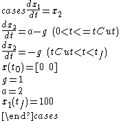
toms tf
toms t
p = tomPhase('p', t, 0, tf, 30);
x0 = {tf
% ODEs and path constraints
a = 2; g = 1;
ceq = {collocate(p1,{
dot(p1,x1p1)
x2p1
dot(p1,x2p1)
a-g})
collocate(p2,{
dot(p2,x1p2)
x2p2
dot(p2,x2p2)
-g})};
% Objective
objective = tCut;
% Link phase
link = {final(p1,x1p1)
initial(p2,x1p2)
final(p1,x2p1)
initial(p2,x2p2)};
%% Solve the problem
options = struct;
options.name = 'One Dim Rocket';
constr = {cbox, cbnd, ceq, link};
solution = ezsolve(objective, constr, x0, options);
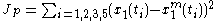
Parameter estimation example Parameter estimation problem
Minimize:
Subject to:
In the code below the problem is solved with a fine grid (10 collocation points). This solution is subsequently fine-tuned using 40 collocation points:
toms t p1 p2
x1meas = [0.264;0.594;0.801;0.959];
tmeas = [1;2;3;5];
In control theory, a bang–bang controller , also known as a hysteresis controller, is a feedback controller that switches abruptly between two states. These controllers may be realized in terms of any element that provides hysteresis...
Chemical engineering is the branch of engineering that deals with physical science , and life sciences with mathematics and economics, to the process of converting raw materials or chemicals into more useful or valuable forms...
A dynamical system is a concept in mathematics where a fixed rule describes the time dependence of a point in a geometrical space. Examples include the mathematical models that describe the swinging of a clock pendulum, the flow of water in a pipe, and the number of fish each springtime in a...
Mechanical engineering is a discipline of engineering that applies the principles of physics and materials science for analysis, design, manufacturing, and maintenance of mechanical systems. It is the branch of engineering that involves the production and usage of heat and mechanical power for the...
In optimal control, problems of singular control are problems that are difficult to solve because a straightforward application of Pontryagin's minimum principle fails to yield a complete solution. Only a few such problems have been solved, such as Merton's portfolio problem in financial economics...
External links
TOMLAB - Developer and distributor of the software.
TomSym - Source transformation engine used in software.


 and constraint function
  that are passed to a Nonlinear programmingNonlinear programmingIn mathematics, nonlinear programming is the process of solving a system of equalities and inequalities, collectively termed constraints, over a set of unknown real variables, along with an objective function to be maximized or minimized, where some of the constraints or the objective function are...