
Monte Carlo method for photon transport
Encyclopedia
Modeling photon propagation with Monte Carlo method
s is a flexible yet rigorous approach to simulate photon transport. In the method, local rules of photon transport are expressed as probability distributions which describe the step size of photon movement between sites of photon-tissue interaction and the angles of deflection in a photon's trajectory when a scattering event occurs. This is equivalent to modeling photon transport analytically by the radiative transfer equation
(RTE), which describes the motion of photons using a differential equation. However, closed-form solutions of the RTE are often not possible; for some geometries, the diffusion approximation
can be used to simplify the RTE, although this, in turn, introduces many inaccuracies, especially near sources and boundaries. In contrast, Monte Carlo simulations can be made arbitrarily accurate by increasing the number of photons traced. For example, see the movie, where a Monte Carlo simulation of a pencil beam
incident on a semi-infinite
medium models both the initial ballistic photon flow and the later diffuse propagation.
The Monte Carlo method is necessarily statistical and therefore requires significant computation time to achieve precision. In addition Monte Carlo simulations can keep track of multiple physical quantities simultaneously, with any desired spatial and temporal resolution. This flexibility makes Monte Carlo modeling a powerful tool. Thus, while computationally inefficient, Monte Carlo methods are often considered the standard for simulated measurements of photon transport for many biomedical applications.
, two-photon
, and optical coherence tomography
) have the ability to image these properties with high spatial resolution, but, since they rely on ballistic photons, their depth penetration is limit to a few millimeters. Imaging deeper into tissues, where photons have been multiply scattered, requires a deeper understanding of the statistical behavior of large numbers of photons in such an environment. Monte Carlo methods provide a flexible framework that has been used by different techniques to reconstruct optical properties deep within tissue. A brief introduction to a few of these techniques is presented here.
is to deliver energy, generally in the form of ionizing radiation, to cancerous tissue while sparing the surrounding normal tissue. Monte carlo modeling is commonly employed in radiation therapy to determine the peripheral dose the patient will experience due to scattering, both from the patient tissue as well as scattering from collimation upstream in the linear accelerator.
(PDT) light is used to activate chemotherapy agents. Due to the nature of PDT, it is useful to use Monte Carlo methods for modeling scattering and absorption in the tissue in order to ensure appropriate levels of light are delivered to activate chemotherapy agents.
in space and time). Responses to arbitrary source geometries can be constructed using the method of Green's functions (or convolution
, if enough spatial symmetry exists). The required parameters are the absorption coefficient, the scattering coefficient, and the scattering phase function. (If boundaries are considered the index of refraction for each medium must also be provided.) Time-resolved responses are found by keeping track of the total elapsed time of the photon's flight using the optical path length
. Responses to sources with arbitrary time profiles can then be modeled through convolution in time.
In our simplified model we use the following variance reduction technique to reduce computational time. Instead of propagating photons individually, we create a photon packet with a specific weight (generally initialized as unity). As the photon interacts in the turbid medium, it will deposit weight due to absorption and the remaining weight will be scattered to other parts of the medium. Any number of variables can be logged along the way, depending on the interest of a particular application. Each photon packet will repeatedly undergo the following numbered steps until it is either terminated, reflected, or transmitted. The process is diagrammed in the schematic to the right. Any number of photon packets can be launched and modeled, until the resulting simulated measurements have the desired signal-to-noise ratio. Note that as Monte Carlo modeling is a statistical process involving random numbers, we will be using the variable ξ throughout as a pseudo-random number
for many calculations.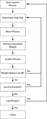
to determine position, along with three direction cosines to determine the direction of propagation. The initial start conditions will vary based on application, however for a pencil beam initialized at the origin, we can set the initial position and direction cosines as follows (isotropic sources can easily be modeled by randomizing the initial direction of each packet):
Monte Carlo method
Monte Carlo methods are a class of computational algorithms that rely on repeated random sampling to compute their results. Monte Carlo methods are often used in computer simulations of physical and mathematical systems...
s is a flexible yet rigorous approach to simulate photon transport. In the method, local rules of photon transport are expressed as probability distributions which describe the step size of photon movement between sites of photon-tissue interaction and the angles of deflection in a photon's trajectory when a scattering event occurs. This is equivalent to modeling photon transport analytically by the radiative transfer equation
Radiative transfer equation and diffusion theory for photon transport in biological tissue
Photon transport in biological tissue can be equivalently modeled numerically with Monte Carlo simulations or analytically by the radiative transfer equation . However, the RTE is difficult to solve without introducing approximations. A common approximation summarized here is the diffusion...
(RTE), which describes the motion of photons using a differential equation. However, closed-form solutions of the RTE are often not possible; for some geometries, the diffusion approximation
Radiative transfer equation and diffusion theory for photon transport in biological tissue
Photon transport in biological tissue can be equivalently modeled numerically with Monte Carlo simulations or analytically by the radiative transfer equation . However, the RTE is difficult to solve without introducing approximations. A common approximation summarized here is the diffusion...
can be used to simplify the RTE, although this, in turn, introduces many inaccuracies, especially near sources and boundaries. In contrast, Monte Carlo simulations can be made arbitrarily accurate by increasing the number of photons traced. For example, see the movie, where a Monte Carlo simulation of a pencil beam
Pencil beam
In optics, a pencil or pencil of rays is a geometric construct used to describe a beam or portion of a beam of electromagnetic radiation or charged particles, typically in the form of a narrow cone or cylinder....
incident on a semi-infinite
Semi-infinite
The term semi-infinite has several related meanings in various branches of pure and applied mathematics. It typically describes objects which are infinite or unbounded in some but not all possible ways.-In ordered structures and Euclidean spaces:...
medium models both the initial ballistic photon flow and the later diffuse propagation.
The Monte Carlo method is necessarily statistical and therefore requires significant computation time to achieve precision. In addition Monte Carlo simulations can keep track of multiple physical quantities simultaneously, with any desired spatial and temporal resolution. This flexibility makes Monte Carlo modeling a powerful tool. Thus, while computationally inefficient, Monte Carlo methods are often considered the standard for simulated measurements of photon transport for many biomedical applications.
Biomedical imaging
The optical properties of biological tissue offer an exciting approach to biomedical imaging. There are many interesting endogenous contrasts, including absorption from blood and melanin and scattering from nerve cells and cancer cell nuclei. In addition, fluorescent probes can be targeted to many different tissues. Microscopy techniques (including confocalConfocal microscopy
Confocal microscopy is an optical imaging technique used to increase optical resolution and contrast of a micrograph by using point illumination and a spatial pinhole to eliminate out-of-focus light in specimens that are thicker than the focal plane. It enables the reconstruction of...
, two-photon
Two-photon excitation microscopy
Two-photon excitation microscopy is a fluorescence imaging technique that allows imaging of living tissue up to a very high depth, that is up to about one millimeter. Being a special variant of the multiphoton fluorescence microscope, it uses red-shifted excitation light which can also excite...
, and optical coherence tomography
Optical coherence tomography
Optical coherence tomography is an optical signal acquisition and processing method. It captures micrometer-resolution, three-dimensional images from within optical scattering media . Optical coherence tomography is an interferometric technique, typically employing near-infrared light...
) have the ability to image these properties with high spatial resolution, but, since they rely on ballistic photons, their depth penetration is limit to a few millimeters. Imaging deeper into tissues, where photons have been multiply scattered, requires a deeper understanding of the statistical behavior of large numbers of photons in such an environment. Monte Carlo methods provide a flexible framework that has been used by different techniques to reconstruct optical properties deep within tissue. A brief introduction to a few of these techniques is presented here.
- Photoacoustic tomography In PAT, diffuse laser light is absorbed which generates a local temperature rise. This local temperature variation in turn generates ultrasound waves via thermoelastic expansion which are detected via an ultrasonic transducer. In practice, a variety of setup parameters are varied (i.e. light wavelength, transducer numerical aperture) and as a result Monte Carlo modeling is a valuable tool for predicting tissue response prior to experimental methods.
- Diffuse optical tomography DOT is an imaging technique that uses an array of near-infrared light sources and detectors to measure optical properties of biological tissues. A variety of contrasts can be measured including the absorption due to oxy- and deoxy-hemoglobin (for functional neuro-imaging or cancer detection) and the concentration of fluorescent probes. In order to reconstruct an image, one must know the manner in which light traveled from a given source to a given detector and how the measurement depends on the distribution and changes in the optical properties (known as the forward model). Due to the highly scattering nature of biological tissue, such paths are complicated and the sensitivity functions are diffuse. The forward model is often generated using Monte Carlo methods.
Radiation therapy
The goal of radiation therapyRadiation therapy
Radiation therapy , radiation oncology, or radiotherapy , sometimes abbreviated to XRT or DXT, is the medical use of ionizing radiation, generally as part of cancer treatment to control malignant cells.Radiation therapy is commonly applied to the cancerous tumor because of its ability to control...
is to deliver energy, generally in the form of ionizing radiation, to cancerous tissue while sparing the surrounding normal tissue. Monte carlo modeling is commonly employed in radiation therapy to determine the peripheral dose the patient will experience due to scattering, both from the patient tissue as well as scattering from collimation upstream in the linear accelerator.
Photodynamic therapy
In Photodynamic therapyPhotodynamic therapy
Photodynamic therapy is used clinically to treat a wide range of medical conditions, including malignant cancers, and is recognised as a treatment strategy which is both minimally invasive and minimally toxic...
(PDT) light is used to activate chemotherapy agents. Due to the nature of PDT, it is useful to use Monte Carlo methods for modeling scattering and absorption in the tissue in order to ensure appropriate levels of light are delivered to activate chemotherapy agents.
Implementation of photon transport in a scattering medium
Presented here is a model of a photon Monte Carlo method in a homogeneous infinite medium, however the model is easily extended for multi-layered media. For an inhomogeneous medium, boundaries must be considered. In addition for a semi-infinite medium (in which photons are considered lost if they exit the top boundary), special consideration must be taken. For more information, please visit the links at the bottom of the page. We will solve the problem using an infinitely small point source (represented analytically as a Dirac delta functionDirac delta function
The Dirac delta function, or δ function, is a generalized function depending on a real parameter such that it is zero for all values of the parameter except when the parameter is zero, and its integral over the parameter from −∞ to ∞ is equal to one. It was introduced by theoretical...
in space and time). Responses to arbitrary source geometries can be constructed using the method of Green's functions (or convolution
Convolution
In mathematics and, in particular, functional analysis, convolution is a mathematical operation on two functions f and g, producing a third function that is typically viewed as a modified version of one of the original functions. Convolution is similar to cross-correlation...
, if enough spatial symmetry exists). The required parameters are the absorption coefficient, the scattering coefficient, and the scattering phase function. (If boundaries are considered the index of refraction for each medium must also be provided.) Time-resolved responses are found by keeping track of the total elapsed time of the photon's flight using the optical path length
Optical path length
In optics, optical path length or optical distance is the product of the geometric length of the path light follows through the system, and the index of refraction of the medium through which it propagates. A difference in optical path length between two paths is often called the optical path...
. Responses to sources with arbitrary time profiles can then be modeled through convolution in time.
In our simplified model we use the following variance reduction technique to reduce computational time. Instead of propagating photons individually, we create a photon packet with a specific weight (generally initialized as unity). As the photon interacts in the turbid medium, it will deposit weight due to absorption and the remaining weight will be scattered to other parts of the medium. Any number of variables can be logged along the way, depending on the interest of a particular application. Each photon packet will repeatedly undergo the following numbered steps until it is either terminated, reflected, or transmitted. The process is diagrammed in the schematic to the right. Any number of photon packets can be launched and modeled, until the resulting simulated measurements have the desired signal-to-noise ratio. Note that as Monte Carlo modeling is a statistical process involving random numbers, we will be using the variable ξ throughout as a pseudo-random number
Pseudorandom number generator
A pseudorandom number generator , also known as a deterministic random bit generator , is an algorithm for generating a sequence of numbers that approximates the properties of random numbers...
for many calculations.
Step 1: Launching a photon packet
In our model, we are ignoring initial specular reflectance associated with entering a medium that is not refractive index matched. With this in mind, we simply need to set the initial position of the photon packet as well as the initial direction. It is convenient to use a global coordinate system. We will use three Cartesian coordinatesCartesian coordinate system
A Cartesian coordinate system specifies each point uniquely in a plane by a pair of numerical coordinates, which are the signed distances from the point to two fixed perpendicular directed lines, measured in the same unit of length...
to determine position, along with three direction cosines to determine the direction of propagation. The initial start conditions will vary based on application, however for a pencil beam initialized at the origin, we can set the initial position and direction cosines as follows (isotropic sources can easily be modeled by randomizing the initial direction of each packet):
-
Step 2: Step size selection and photon packet movement
The step size, s, is the distance the photon packet travels between interaction sites. There are a variety of methods for step size selection. Below is a basic form of photon step size selection (derived using the inverse distribution method and the Beer–Lambert law) from which we use for our homogeneous model:
Once a step size is selected, the photon packet is propagated by a distance s in a direction defined by the direction cosines. This is easily accomplished by simply updating the coordinates as follows:
-
Step 3: Absorption and scattering
A portion of the photon weight is absorbed at each interaction site. This fraction of the weight is determined as follows:
The weight fraction can then be recorded in an array if an absorption distribution is of interest for the particular study. The weight of the photon packet must then be updated as follows:
Following absorption, the photon packet is scattered. The weighted average of the cosine of the photon scattering angle is known as scattering anisotropy (g), which has a value between −1 and 1. If the optical anisotropy is 0, this generally indicates that the scattering is isotropic. If g approaches a value of 1 this indicates that the scattering is primarily in the forward direction. In order to determine the new direction of the photon packet (and hence the photon direction cosines), we need to know the scattering phase function. Often the Henyey-Greenstein phase function is used. Then the scattering angle, θ, is determined using the following formula.
-
And, the polar angle φ is generally assumed to be uniformly distributed between 0 and . Based on this assumption, we can set:
-

Based on these angles and the original direction cosines, we can find a new set of direction cosines. The new propagation direction can be represented in the global coordinate system as follows:
-
For a special case-

use
-
C-code:
********************** Indicatrix *********************
New direction cosines after scattering by angle teta, fi.
See http://en.wikipedia.org/wiki/Monte_Carlo_method_for_photon_transport
mux new=(sin(teta)*(mux*muz*cos(fi)-muy*sin(fi)))/sqrt(1-muz^2)+mux*cos(teta)
muy new=(sin(teta)*(muy*muz*cos(fi)+mux*sin(fi)))/sqrt(1-muz^2)+muy*cos(teta)
muz new= - sqrt(1-muz^2)*sin(teta)*cos(fi)+muz*cos(teta)
---------------------------------------------------------
Input:
muxs,muys,muzs - direction cosine before collision
muteta, fi - cosine of polar angle and the azimuthal angle
---------------------------------------------------------
Output:
muxd,muyd,muzd - direction cosine after collision
---------------------------------------------------------
void Indicatrix(double muxs,double muys,double muzs,double muteta,double fi,double *muxd,double *muyd,double *muzd){
double costeta=muteta;
double sinteta=sqrt(1.0-costeta*costeta); // sin(theta)
double sinfi=sin(fi);
double cosfi=cos(fi);
if(muzs1.0){
*muxd=sinteta*cosfi;
*muyd=sinteta*sinfi;
*muzd=costeta;
return;
}
{
double denom=sqrt(1.0-muzs*muzs);
double muzcosfi=muzs*cosfi;
*muxd=sinteta*(muxs*muzcosfi-muys*sinfi)/denom+muxs*costeta;
*muyd=sinteta*(muys*muzcosfi+muxs*sinfi)/denom+muys*costeta;
*muzd=-denom*sinteta*cosfi+muzs*costeta;
}
}
Step 4: Photon termination
If a photon packet has experienced many interactions, for most applications the weight left in the packet is of little consequence. As a result it is necessary to determine a means for terminating photon packets of sufficiently small weight. A simple method would use a threshold, and if the weight of the photon packet is below the threshold, the packet is considered dead. The aforementioned method is limited as it does not conserve energy. To keep total energy constant, a Russian rouletteRussian rouletteRussian roulette is a potentially lethal game of chance in which participants place a single round in a revolver, spin the cylinder, place the muzzle against their head and pull the trigger...
technique is often employed for photons below a certain weight threshold. This technique uses a roulette constant m to determine whether or not the photon will survive. The photon packet has one chance in m to survive, in which case it will be given a new weight of mW where W is the initial weight (this new weight, on average, conserves energy). All other times, the photon weight is set to 0 and the photon is terminated. This is expressed mathematically below:
-

Graphics Processing Units (GPU) and fast Monte Carlo simulations of photon transport
Monte Carlo simulation of photon migration in turbid media is a highly parallelable problem, where a large number of photons are propagated independently, but according to identical rules and different random number sequences. The parallel nature of this special type of Monte Carlo simulation renders it highly suitable for execution on a graphics processing unit (GPU). The release of programmable GPUs started such a development, and since 2008 there are a few reports on the use of GPU for high-speed Monte Carlo simulation of photon migration .
Acceleration of Monte Carlo simulation using GPU cluster
Monte Carlo simulation is of great significance in simulating the light propagation in tissues, which quantifies the light delivered to the treated tissue and is an important factor for improving clinical results. However, Monte Carlo simulation is very time-consuming because of the extensive computational burden. It limits the practical application of Monte Carlo method greatly. To improve the performance of Monte Carlo simulation for photon transport in turbid media, a new version of Monte Carlo program for simulation of light transport in multi-layered tissues is developed base on the GPU Cluster. it is called "GPU Cluster MCML" in simple words. It has the same function as Lihong Wang and Steven L. Jacques' "MCML" running on the CPU. In the "GPU Cluster MCML", Distributed Computing of GPU Clusters installed in different personal computers within a local area network (LAN) are employed to accelerating the simulation greatly.
The executable for tests can be download from the website(Monte Carlo Simulation of Light Transport in Multi-layered Turbid Media Based on GPU Clusters
):
http://bmp.hust.edu.cn/GPU_Cluster/GPU_Cluster_MCML.HTM
See also
Links to other Monte Carlo resources- Radiative transfer equation and diffusion theory for photon transport in biological tissueRadiative transfer equation and diffusion theory for photon transport in biological tissuePhoton transport in biological tissue can be equivalently modeled numerically with Monte Carlo simulations or analytically by the radiative transfer equation . However, the RTE is difficult to solve without introducing approximations. A common approximation summarized here is the diffusion...
- Monte Carlo methodMonte Carlo methodMonte Carlo methods are a class of computational algorithms that rely on repeated random sampling to compute their results. Monte Carlo methods are often used in computer simulations of physical and mathematical systems...
- Convolution for optical broad-beam responses in scattering mediaConvolution for optical broad-beam responses in scattering mediaPhoton transport theories, such as the Monte Carlo method, are commonly used to model light propagation in tissue. The responses to a pencil beam incident on a scattering medium are referred to as Green’s functions or impulse responses. Photon transport methods can be directly used to compute...
- Monte Carlo methods for electron transportMonte Carlo methods for electron transportThe Monte Carlo method for electron transport is a semiclassical Monte Carlo approach of modeling semiconductor transport. Assuming the carrier motion consists of free flights interrupted by scattering mechanisms, a computer is utilized to simulate the trajectories of particles as they move across...
- Optical Imaging Laboratory at Washington University in St. Louis (MCML)
- Oregon Medical Laser Center
- Photon migration Monte Carlo research at Lund University, Sweden GPU acceleration of Monte Carlo simualtions and scalable Monte Carlo. Open source code for download.
- Biophotonics & Biomedical Imaging Research Group, University of Otago, Dunedin, New Zealand Online GPU-accelerated multipurpose Monte Carlo simulation tool for the needs of Biophotonics and Biomedical Optics. The tool is free to use in research and non-commercial activities.
- Radiative transfer equation and diffusion theory for photon transport in biological tissue
-
-
-
-
-
-
-


