
Cubic Hermite spline
Encyclopedia
In the mathematical
subfield of numerical analysis
a cubic Hermite spline (also called cspline), named in honor of Charles Hermite
, is a third-degree spline
with each polynomial
of the spline in Hermite form. The Hermite form consists of two control points and two control tangents for each polynomial.
For interpolation on a grid with points for
for  , interpolation is performed on one subinterval
  at a time (given that tangent values are predetermined). The subinterval
  is normalized to
  via
via  .
.
 , given a starting point p0 at
  and an ending point p1 at
  with starting tangent m0 at
  and ending tangent m1 at
  , the polynomial can be defined by
 where t ∈ [0, 1].
 in the interval
  can now be done with the formula
with and
and  refers to the basis functions, defined below. Note that the tangent values have been scaled by
  compared to the equation on the unit interval.
Proof:
Let be another third degree polynomial satisfying the given boundary conditions. Define
  . Since both
  and
and  are third degree polynomials,
  is at most a third degree polynomial. Furthermore:
 (We assume both
  and
and  satisfy the boundary conditions)
So must be of the form:


We know furthermore that:


Putting and
and  together, we deduce that
  and
and  , thus

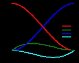
where are Hermite basis functions.
These can be written in different ways, each way revealing different properties.
|-
!
! expanded
! factorized
! Bernstein
|-
|
|
|
|
|-
|
|
|
|
|-
|
|
|
|
|-
|
|
|
|
|}>
The "expanded" column shows the representation used in the definition above.
The "factorized" column shows immediately, that and
and  are zero at the boundaries.
You can further conclude
that and
and  have a zero of multiplicity 2 at 0
and and
and  have such a zero at 1,
thus they have slope 0 at those boundaries.
The "Bernstein" column shows the decomposition of the Hermite basis functions into Bernstein polynomial
s of order 3:

Using this connection you can express cubic Hermite interpolation in terms of cubic Bézier curve
s
with respect to the four values
and do Hermite interpolation using the de Casteljau algorithm.
It shows that in a cubic Bézier patch the two control points in the middle
determine the tangents of the interpolation curve at the respective outer points.
 for
for  , can be interpolated by applying the above procedure on each interval, where the tangents are chosen in a sensible manner, meaning that the tangents for intervals sharing endpoints are equal. The interpolated curve then consists of piecewise cubic Hermite splines, and is globally continuously differentiable in
  .
.
The choice of tangents is non-unique, and there are several options available.

for internal points , and one-sided difference at the endpoints of the data set.
 A cardinal spline is obtained if
is used to calculate the tangents. The parameter is a tension parameter that must be in the interval
  . In some sense, this can be interpreted as the "length" of the tangent.
  will yield all zero tangents, and
  yields a Catmull–Rom spline.
For tangents chosen to be
a Catmull–Rom spline is obtained, being a special case of a cardinal spline.
The curve is named after Edwin Catmull
and Raphael (Raphie) Rom. In computer graphics
, Catmull–Rom splines are frequently used to get smooth interpolated motion between key frame
s. For example, most camera path animations generated from discrete key-frames are handled using Catmull–Rom splines. They are popular mainly for being relatively easy to compute, guaranteeing that each key frame position will be hit exactly, and also guaranteeing that the tangents of the generated curve are continuous over multiple segments.
 ,
,  and
and  , with three parameters possible, tension, bias and a continuity parameter.
of a monotonic
data set, the interpolated function will not necessarily be monotonic, but monotonicity can be preserved by adjusting the tangents.

for , where the left-hand vector is independent of the p.
This writing is relevant for tricubic interpolation
, where one optimization requires you to compute CINTx sixteen times with the same x and different p.
Mathematics
Mathematics is the study of quantity, space, structure, and change. Mathematicians seek out patterns and formulate new conjectures. Mathematicians resolve the truth or falsity of conjectures by mathematical proofs, which are arguments sufficient to convince other mathematicians of their validity...
subfield of numerical analysis
Numerical analysis
Numerical analysis is the study of algorithms that use numerical approximation for the problems of mathematical analysis ....
a cubic Hermite spline (also called cspline), named in honor of Charles Hermite
Charles Hermite
Charles Hermite was a French mathematician who did research on number theory, quadratic forms, invariant theory, orthogonal polynomials, elliptic functions, and algebra....
, is a third-degree spline
Spline (mathematics)
In mathematics, a spline is a sufficiently smooth piecewise-polynomial function. In interpolating problems, spline interpolation is often preferred to polynomial interpolation because it yields similar results, even when using low-degree polynomials, while avoiding Runge's phenomenon for higher...
with each polynomial
Polynomial
In mathematics, a polynomial is an expression of finite length constructed from variables and constants, using only the operations of addition, subtraction, multiplication, and non-negative integer exponents...
of the spline in Hermite form. The Hermite form consists of two control points and two control tangents for each polynomial.
For interpolation on a grid with points
for , interpolation is performed on one subinterval at a time (given that tangent values are predetermined). The subinterval is normalized to via .Unit interval (0, 1)
On the unit interval, given a starting point p0 at and an ending point p1 at with starting tangent m0 at and ending tangent m1 at , the polynomial can be defined byInterpolation on (xk, xk+1)
Interpolating in the interval can now be done with the formulawith
and refers to the basis functions, defined below. Note that the tangent values have been scaled by compared to the equation on the unit interval.Uniqueness
The formulae specified above are guaranteed to produce a unique path between the two points.Proof:
Let
be another third degree polynomial satisfying the given boundary conditions. Define . Since both and are third degree polynomials, is at most a third degree polynomial. Furthermore: (We assume both and satisfy the boundary conditions)So
must be of the form:We know furthermore that:
Putting
and together, we deduce that and , thus Representations
We can write the interpolation polynomial aswhere
are Hermite basis functions.These can be written in different ways, each way revealing different properties.
!
! expanded
! factorized
! Bernstein
|-
|
|
|
|
|-
|
|
|
|
|-
|
|
|
|
|-
|
|
|
|
|}>
The "expanded" column shows the representation used in the definition above.
The "factorized" column shows immediately, that
and are zero at the boundaries.You can further conclude
that
and have a zero of multiplicity 2 at 0and
and have such a zero at 1,thus they have slope 0 at those boundaries.
The "Bernstein" column shows the decomposition of the Hermite basis functions into Bernstein polynomial
Bernstein polynomial
In the mathematical field of numerical analysis, a Bernstein polynomial, named after Sergei Natanovich Bernstein, is a polynomial in the Bernstein form, that is a linear combination of Bernstein basis polynomials....
s of order 3:
Using this connection you can express cubic Hermite interpolation in terms of cubic Bézier curve
Bézier curve
A Bézier curve is a parametric curve frequently used in computer graphics and related fields. Generalizations of Bézier curves to higher dimensions are called Bézier surfaces, of which the Bézier triangle is a special case....
s
with respect to the four values
and do Hermite interpolation using the de Casteljau algorithm.
It shows that in a cubic Bézier patch the two control points in the middle
determine the tangents of the interpolation curve at the respective outer points.
Interpolating a data set
A data set, for , can be interpolated by applying the above procedure on each interval, where the tangents are chosen in a sensible manner, meaning that the tangents for intervals sharing endpoints are equal. The interpolated curve then consists of piecewise cubic Hermite splines, and is globally continuously differentiable in .The choice of tangents is non-unique, and there are several options available.
Finite difference
The simplest choice is the three-point difference, not requiring constant interval lengths,for internal points
, and one-sided difference at the endpoints of the data set.Cardinal spline
is used to calculate the tangents. The parameter
is a tension parameter that must be in the interval . In some sense, this can be interpreted as the "length" of the tangent. will yield all zero tangents, and yields a Catmull–Rom spline.Catmull–Rom spline
For tangents chosen to be
a Catmull–Rom spline is obtained, being a special case of a cardinal spline.
The curve is named after Edwin Catmull
Edwin Catmull
Dr. Edwin Earl Catmull, Ph.D. is a computer scientist and current president of Walt Disney Animation Studios and Pixar Animation Studios. As a computer scientist, Catmull has contributed to many important developments in computer graphics....
and Raphael (Raphie) Rom. In computer graphics
Computer graphics
Computer graphics are graphics created using computers and, more generally, the representation and manipulation of image data by a computer with help from specialized software and hardware....
, Catmull–Rom splines are frequently used to get smooth interpolated motion between key frame
Key frame
A key frame in animation and filmmaking is a drawing that defines the starting and ending points of any smooth transition. They are called "frames" because their position in time is measured in frames on a strip of film...
s. For example, most camera path animations generated from discrete key-frames are handled using Catmull–Rom splines. They are popular mainly for being relatively easy to compute, guaranteeing that each key frame position will be hit exactly, and also guaranteeing that the tangents of the generated curve are continuous over multiple segments.
Kochanek–Bartels spline
A Kochanek–Bartels spline is a further generalization on how to choose the tangents given the data points, and , with three parameters possible, tension, bias and a continuity parameter.Monotone cubic interpolation
If a cubic Hermite spline of any of the above listed types is used for interpolationInterpolation
In the mathematical field of numerical analysis, interpolation is a method of constructing new data points within the range of a discrete set of known data points....
of a monotonic
Monotonic function
In mathematics, a monotonic function is a function that preserves the given order. This concept first arose in calculus, and was later generalized to the more abstract setting of order theory....
data set, the interpolated function will not necessarily be monotonic, but monotonicity can be preserved by adjusting the tangents.
Interpolation on the unit interval without exact derivatives
Given p-1, p0, p1 and p2 as the values that the function should take on at -1, 0, 1 and 2, we can use centered differences instead of exact derivatives. Thus the Catmull–Rom spline isfor
, where the left-hand vector is independent of the p.This writing is relevant for tricubic interpolation
Tricubic interpolation
In the mathematical subfield numerical analysis, tricubic interpolation is a method for obtaining values at arbitrary points in 3D space of a function defined on a regular grid...
, where one optimization requires you to compute CINTx sixteen times with the same x and different p.
See also
- Bicubic interpolationBicubic interpolationIn mathematics, bicubic interpolation is an extension of cubic interpolation for interpolating data points on a two dimensional regular grid. The interpolated surface is smoother than corresponding surfaces obtained by bilinear interpolation or nearest-neighbor interpolation...
, a generalization to two dimensions - Tricubic interpolationTricubic interpolationIn the mathematical subfield numerical analysis, tricubic interpolation is a method for obtaining values at arbitrary points in 3D space of a function defined on a regular grid...
, a generalization to three dimensions - Hermite interpolationHermite interpolationIn numerical analysis, Hermite interpolation, named after Charles Hermite, is a method of interpolating data points as a polynomial function. The generated Hermite polynomial is closely related to the Newton polynomial, in that both are derived from the calculation of divided differences.Unlike...
- Multivariate interpolationMultivariate interpolationIn numerical analysis, multivariate interpolation or spatial interpolation is interpolation on functions of more than one variable.The function to be interpolated is known at given points and the interpolation problem consist of yielding values at arbitrary points .-Regular grid:For function...
- Spline interpolationSpline interpolationIn the mathematical field of numerical analysis, spline interpolation is a form of interpolation where the interpolant is a special type of piecewise polynomial called a spline. Spline interpolation is preferred over polynomial interpolation because the interpolation error can be made small even...
External links
- Spline Curves, Prof. Donald H. House Clemson UniversityClemson UniversityClemson University is an American public, coeducational, land-grant, sea-grant, research university located in Clemson, South Carolina, United States....
- Multi-dimensional Hermite Interpolation and Approximation, Prof. Chandrajit Bajaja, Purdue UniversityPurdue UniversityPurdue University, located in West Lafayette, Indiana, U.S., is the flagship university of the six-campus Purdue University system. Purdue was founded on May 6, 1869, as a land-grant university when the Indiana General Assembly, taking advantage of the Morrill Act, accepted a donation of land and...
- Introduction to Catmull-Rom Splines, MVPs.org
- Interpolating Cardinal and Catmull-Rom splines
- Interpolation methods: linear, cosine, cubic and hermite (with C sources)
- Common Spline Equations