

Tricubic interpolation
Encyclopedia
Numerical analysis
Numerical analysis is the study of algorithms that use numerical approximation for the problems of mathematical analysis ....
, tricubic interpolation is a method for obtaining values at arbitrary points in 3D space
Three-dimensional space
Three-dimensional space is a geometric 3-parameters model of the physical universe in which we live. These three dimensions are commonly called length, width, and depth , although any three directions can be chosen, provided that they do not lie in the same plane.In physics and mathematics, a...
of a function defined on a regular grid
Regular grid
A regular grid is a tessellation of n-dimensional Euclidean space by congruent parallelotopes . Grids of this type appear on graph paper and may be used in finite element analysis as well as finite volume methods and finite difference methods...
. The approach involves approximating the function locally by an expression of the form
This form has 64 coefficients
 ; requiring the function to have a given value or given directional derivative
Directional derivative
In mathematics, the directional derivative of a multivariate differentiable function along a given vector V at a given point P intuitively represents the instantaneous rate of change of the function, moving through P in the direction of V...
at a point places one linear constraint on the 64 coefficients.
The term tricubic interpolation is used in more than one context; some experiments measure both the value of a function and its spatial derivatives, and it is desirable to interpolate preserving the values and the measured derivatives at the grid points. Those provide 32 constraints on the coefficients, and another 32 constraints can be provided by requiring smoothness of higher derivatives; see for details.
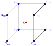
In other contexts, we can obtain the 64 coefficients by considering a 3x3x3 grid of small cubes surrounding the cube inside which we evaluate the function, and fitting the function at the 64 points on the corners of this grid.
The cubic interpolation article indicates that the method is equivalent to a sequential application of one dimensional cubic interpolators. Indeed, define
 as the value of the unique cubic polynomial with
  evaluated at x. We have
  for some vector
  which is a function of x alone. Therefore, the tricubic interpolator is equivalent to
-

At first glance, it might seem more convenient to use the 21 calls to described above instead of the
  matrix described in Lekien and Marsden. However, proper implementation using a sparse format for the matrix (that is fairly sparse) makes the later more efficient. This aspect is even much more pronounced when interpolation is needed at several locations inside the same cube. In this case, the
  matrix is used once to compute the interpolation coefficients for the entire cube. The coefficients are then stored and used for interpolation at any location inside the cube. In comparison, sequential use of one-dimensional integrators
  performs extremely poorly for repeated interpolations because each computational step must be repeated for each new location.
External links