

Runge–Kutta methods
Encyclopedia
In numerical analysis
, the Runge–Kutta methods (ˌʁʊŋəˈkʊta) are an important family of implicit and explicit iterative methods for the approximation of solutions of ordinary differential equation
s. These techniques were developed around 1900 by the German mathematicians C. Runge and M.W. Kutta
.
See the article on numerical ordinary differential equations
for more background and other methods. See also List of Runge–Kutta methods.
Let an initial value problem
be specified as follows.
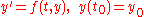
In words, what this means is that the rate at which y changes is a function of y and of t (time). At the start, time is and y is
  .
.
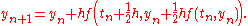
The RK4 method for this problem is given by the following equations:
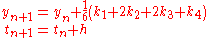
where is the RK4 approximation of
  , and
, and
Thus, the next value ( ) is determined by the present value (
 ) plus the weighted average of 4 deltas, where each delta is the product of the size of the interval (
 ) and an estimated slope
: .
.
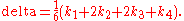
In averaging the four deltas, greater weight is given to the deltas at the midpoint:
The RK4 method is a fourth-order method, meaning that the error per step is on the order of
 , while the total accumulated error has order
  .
.
Note that the above formulae are valid for both scalar- and vector-valued functions (i.e., can be a vector and
  an operator). For example one can integrate the time independent Schrödinger equation using the Hamiltonian operator as function
  .
.
Also note that if is independent of
  , so that the differential equation is equivalent to a simple integral, then RK4 is Simpson's rule
.
Runge–Kutta methods is a generalization
of the RK4 method mentioned above. It is given by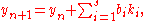
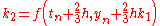
where


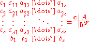
To specify a particular method, one needs to provide the integer s (the number of stages), and the coefficients aij (for 1 ≤ j < i ≤ s), bi (for i = 1, 2, ..., s) and ci (for i = 2, 3, ..., s). These data are usually arranged in a mnemonic device, known as a Butcher tableau (after John C. Butcher
):
The Runge–Kutta method is consistent if
There are also accompanying requirements if we require the method to have a certain order p, meaning that the local truncation error is O(hp+1). These can be derived from the definition of the truncation error itself. For example, a 2-stage method has order 2 if b1 + b2 = 1, b2c2 = 1/2, and b2a21 = 1/2.
However, the simplest Runge–Kutta method is the (forward) Euler method
, given by the formula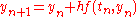 . This is the only consistent explicit Runge–Kutta method with one stage. The corresponding tableau is:
An example of a second-order method with two stages is provided by the midpoint method
The corresponding tableau is:
Note that this 'midpoint' method is not the optimal RK2 method. An alternative is provided by Heun's method
, where the 1/2's in the tableau above are replaced by 1's and the b's row is [1/2, 1/2].
In fact, a family of RK2 methods is

where is the mid-point method and
  is Heun's method
.
If one wants to minimize the truncation error, the method below should be used (Atkinson p. 423). Other important methods are Fehlberg
, Cash-Karp and Dormand-Prince. To use unequally spaced intervals requires an adaptive stepsize
method.
to solve the initial-value problem
with step size h=0.025.
The tableau above yields the equivalent corresponding equations below defining the method

The numerical solutions correspond to the underlined values. Note that has been calculated to avoid recalculation in the
  s.
s.
 and one with order
  .
.
The lower-order step is given by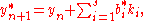
where the are the same as for the higher order method. Then the error is
which is .
.
The Butcher Tableau for this kind of method is extended to give the values of :
:
The Runge–Kutta–Fehlberg method
has two methods of orders 5 and 4. Its extended Butcher Tableau is:
However, the simplest adaptive Runge–Kutta method involves combining the Heun method, which is order 2, with the Euler method, which is order 1. Its extended Butcher Tableau is:
The error estimate is used to control the stepsize.
Other adaptive Runge–Kutta methods are the Bogacki–Shampine method
(orders 3 and 2), the Cash–Karp method
and the Dormand–Prince method
(both with orders 5 and 4).
 is not necessarily lower triangular:
The approximate solution to the initial value problem reflects the greater number of coefficients:
Due to the fullness of the matrix , the evaluation of each
  is now considerably involved and dependent on the specific function
  . Despite the difficulties, implicit methods are of great importance due to their high (possibly unconditional) stability, which is especially important in the solution of partial differential equations
. The simplest example of an implicit Runge–Kutta method is the backward Euler method:

The Butcher Tableau for this is simply:

It can be difficult to make sense of even this simple implicit method, as seen from the expression for :
:

In this case, the awkward expression above can be simplified by noting that

so that

from which

follows. Though simpler than the "raw" representation before manipulation, this is an implicit relation so that the actual solution is problem dependent. Multistep implicit methods have been used with success by some researchers. The combination of stability, higher order accuracy with fewer steps, and stepping that depends only on the previous value makes them attractive; however the complicated problem-specific implementation and the fact that must often be approximated iteratively means that they are not common.

Numerical analysis
Numerical analysis is the study of algorithms that use numerical approximation for the problems of mathematical analysis ....
, the Runge–Kutta methods (ˌʁʊŋəˈkʊta) are an important family of implicit and explicit iterative methods for the approximation of solutions of ordinary differential equation
Ordinary differential equation
In mathematics, an ordinary differential equation is a relation that contains functions of only one independent variable, and one or more of their derivatives with respect to that variable....
s. These techniques were developed around 1900 by the German mathematicians C. Runge and M.W. Kutta
Martin Wilhelm Kutta
Martin Wilhelm Kutta was a German mathematician.Kutta was born in Pitschen, Upper Silesia . He attended the University of Breslau from 1885 to 1890, and continued his studies in Munich until 1894, where he became the assistant of Walther Franz Anton von Dyck. From 1898, he spent a year at the...
.
See the article on numerical ordinary differential equations
Numerical ordinary differential equations
Numerical ordinary differential equations is the part of numerical analysis which studies the numerical solution of ordinary differential equations...
for more background and other methods. See also List of Runge–Kutta methods.
Common fourth-order Runge–Kutta method
One member of the family of Runge–Kutta methods is so commonly used that it is often referred to as "RK4", "classical Runge-Kutta method" or simply as "the Runge–Kutta method".Let an initial value problem
Initial value problem
In mathematics, in the field of differential equations, an initial value problem is an ordinary differential equation together with a specified value, called the initial condition, of the unknown function at a given point in the domain of the solution...
be specified as follows.
In words, what this means is that the rate at which y changes is a function of y and of t (time). At the start, time is
and y is .The RK4 method for this problem is given by the following equations:
where
is the RK4 approximation of , andThus, the next value (
) is determined by the present value () plus the weighted average of 4 deltas, where each delta is the product of the size of the interval () and an estimated slopeSlope
In mathematics, the slope or gradient of a line describes its steepness, incline, or grade. A higher slope value indicates a steeper incline....
:
.-
 is the delta based on the slope at the beginning of the interval, using
  , ( Euler's method ) ;
 -
 is the delta based on the slope at the midpoint of the interval, using
  1/2
1/2  ;
; -
 is again the delta based on the slope at the midpoint, but now using
  1/2
1/2  ;
; -
 is the delta based on the slope at the end of the interval, using
  .
.
In averaging the four deltas, greater weight is given to the deltas at the midpoint:
The RK4 method is a fourth-order method, meaning that the error per step is on the order of
Big O notation
In mathematics, big O notation is used to describe the limiting behavior of a function when the argument tends towards a particular value or infinity, usually in terms of simpler functions. It is a member of a larger family of notations that is called Landau notation, Bachmann-Landau notation, or...
, while the total accumulated error has order .Note that the above formulae are valid for both scalar- and vector-valued functions (i.e.,
can be a vector and an operator). For example one can integrate the time independent Schrödinger equation using the Hamiltonian operator as function .Also note that if
is independent of , so that the differential equation is equivalent to a simple integral, then RK4 is Simpson's ruleSimpson's rule
In numerical analysis, Simpson's rule is a method for numerical integration, the numerical approximation of definite integrals. Specifically, it is the following approximation:...
.
Explicit Runge–Kutta methods
The family of explicitExplicit and implicit methods
Explicit and implicit methods are approaches used in numerical analysis for obtaining numerical solutions of time-dependent ordinary and partial differential equations, as is required in computer simulations of physical processes....
Runge–Kutta methods is a generalization
Generalization
A generalization of a concept is an extension of the concept to less-specific criteria. It is a foundational element of logic and human reasoning. Generalizations posit the existence of a domain or set of elements, as well as one or more common characteristics shared by those elements. As such, it...
of the RK4 method mentioned above. It is given by
where
-
-
- (Note: the above equations have different but equivalent definitions in different texts).


To specify a particular method, one needs to provide the integer s (the number of stages), and the coefficients aij (for 1 ≤ j < i ≤ s), bi (for i = 1, 2, ..., s) and ci (for i = 2, 3, ..., s). These data are usually arranged in a mnemonic device, known as a Butcher tableau (after John C. Butcher
John C. Butcher
John Charles Butcher is a mathematician who specialises in numerical methods for the solution of ordinary differential equations. Butcher works on multistage methods for initial value problems, such as Runge-Kutta and general linear methods...
):
| 0 | |||||
|  |
 |
||||
|  |
 |
 |
|||
|  |
 |
 |
|||
|  |
 |
 |
 |
 |
|
| | |  |
 |
 |
 |
 |
The Runge–Kutta method is consistent if
There are also accompanying requirements if we require the method to have a certain order p, meaning that the local truncation error is O(hp+1). These can be derived from the definition of the truncation error itself. For example, a 2-stage method has order 2 if b1 + b2 = 1, b2c2 = 1/2, and b2a21 = 1/2.
Examples
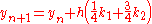
The RK4 method falls in this framework. Its tableau is:| 0 | ||||
| | 1/2 | 1/2 | |||
| | 1/2 | 0 | 1/2 | ||
| | 1 | 0 | 0 | 1 | |
| | | 1/6 | 1/3 | 1/3 | 1/6 |
However, the simplest Runge–Kutta method is the (forward) Euler method
Euler integration
In mathematics and computational science, the Euler method, named after Leonhard Euler, is a first-order numerical procedure for solving ordinary differential equations with a given initial value...
, given by the formula
. This is the only consistent explicit Runge–Kutta method with one stage. The corresponding tableau is:| 0 | |
| | | 1 |
An example of a second-order method with two stages is provided by the midpoint method
Midpoint method
In numerical analysis, a branch of applied mathematics, the midpoint method is a one-step method for solving the differential equation y' = f, \quad y = y_0...
The corresponding tableau is:
| 0 | ||
| | 1/2 | 1/2 | |
| | | 0 | 1 |
Note that this 'midpoint' method is not the optimal RK2 method. An alternative is provided by Heun's method
Heun's method
In mathematics and computational science, Heun's method may refer to the improved or modified Euler's method , or a similar two-stage Runge–Kutta method. It is named after Karl L. W. M. Heun and is a numerical procedure for solving ordinary differential equations with a given initial value...
, where the 1/2's in the tableau above are replaced by 1's and the b's row is [1/2, 1/2].
In fact, a family of RK2 methods is
where
is the mid-point method and is Heun's methodHeun's method
In mathematics and computational science, Heun's method may refer to the improved or modified Euler's method , or a similar two-stage Runge–Kutta method. It is named after Karl L. W. M. Heun and is a numerical procedure for solving ordinary differential equations with a given initial value...
.
If one wants to minimize the truncation error, the method below should be used (Atkinson p. 423). Other important methods are Fehlberg
Runge–Kutta–Fehlberg method
In mathematics, the Runge–Kutta–Fehlberg method is an algorithm of numerical analysis for the numerical solution of ordinary differential equations. It was developed by the German mathematician Erwin Fehlberg and is based on the class of Runge–Kutta methods...
, Cash-Karp and Dormand-Prince. To use unequally spaced intervals requires an adaptive stepsize
Adaptive stepsize
Adaptive stepsize is a technique in numerical analysis used for many problems, but mainly for integration. It can be used for both normal integration , or the process of solving an ordinary differential equation. This article focuses on the latter...
method.
Usage
The following is an example usage of a two-stage explicit Runge–Kutta method:| 0 | ||
| | 2/3 | 2/3 | |
| | | 1/4 | 3/4 |
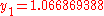
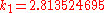
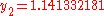
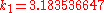
to solve the initial-value problem
with step size h=0.025.
The tableau above yields the equivalent corresponding equations below defining the method
 |
|||
 |
|||
 |
|||
 |
 |
 |
|
 |
|||
 |
|||
 |
 |
 |
|
 |
|||
 |
|||
 |
 |
 |
|
 |
|||
 |
|||
 |
 |
 |
|
 |
|||
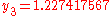
The numerical solutions correspond to the underlined values. Note that
has been calculated to avoid recalculation in the s.Adaptive Runge–Kutta methods
The adaptive methods are designed to produce an estimate of the local truncation error of a single Runge–Kutta step. This is done by having two methods in the tableau, one with order and one with order .The lower-order step is given by
where the
are the same as for the higher order method. Then the error iswhich is
.The Butcher Tableau for this kind of method is extended to give the values of
:| 0 | |||||
|  |
 |
||||
|  |
 |
 |
|||
|  |
 |
 |
|||
|  |
 |
 |
 |
 |
|
| | |  |
 |
 |
 |
 |
| | |  |
 |
 |
 |
 |
The Runge–Kutta–Fehlberg method
Runge–Kutta–Fehlberg method
In mathematics, the Runge–Kutta–Fehlberg method is an algorithm of numerical analysis for the numerical solution of ordinary differential equations. It was developed by the German mathematician Erwin Fehlberg and is based on the class of Runge–Kutta methods...
has two methods of orders 5 and 4. Its extended Butcher Tableau is:
| 0 | ||||||
| | 1/4 | 1/4 | |||||
| | 3/8 | 3/32 | 9/32 | ||||
| | 12/13 | 1932/2197 | −7200/2197 | 7296/2197 | |||
| | 1 | 439/216 | −8 | 3680/513 | -845/4104 | ||
| | 1/2 | −8/27 | 2 | −3544/2565 | 1859/4104 | −11/40 | |
| | | 16/135 | 0 | 6656/12825 | 28561/56430 | −9/50 | 2/55 |
| | | 25/216 | 0 | 1408/2565 | 2197/4104 | −1/5 | 0 |
However, the simplest adaptive Runge–Kutta method involves combining the Heun method, which is order 2, with the Euler method, which is order 1. Its extended Butcher Tableau is:
| 0 | ||
| | 1 | 1 | |
| | | 1/2 | 1/2 |
| | | 1 | 0 |
The error estimate is used to control the stepsize.
Other adaptive Runge–Kutta methods are the Bogacki–Shampine method
Bogacki–Shampine method
The Bogacki–Shampine method is a method for the numerical solution of ordinary differential equations, that was proposed by Przemyslaw Bogacki and Lawrence F. Shampine in 1989 . The Bogacki–Shampine method is a Runge–Kutta method of order three with four stages with the First Same As Last ...
(orders 3 and 2), the Cash–Karp method
Cash–Karp method
In numerical analysis, the Cash–Karp method is a method for solving ordinary differential equations . It was proposed by Professor Jeff R. Cash from Imperial College London and Alan H. Karp from IBM Scientific Center. The method is a member of the Runge–Kutta family of ODE solvers...
and the Dormand–Prince method
Dormand–Prince method
In numerical analysis, the Dormand–Prince method, or DOPRI method, is a method for solving ordinary differential equations . The method is a member of the Runge–Kutta family of ODE solvers. More specifically, it uses six function evaluations to calculate fourth- and fifth-order accurate solutions...
(both with orders 5 and 4).
Implicit Runge–Kutta methods
The implicit methods are more general than the explicit ones. The distinction shows up in the Butcher Tableau: for an implicit method, the coefficient matrix is not necessarily lower triangular:The approximate solution to the initial value problem reflects the greater number of coefficients:
Due to the fullness of the matrix
, the evaluation of each is now considerably involved and dependent on the specific function . Despite the difficulties, implicit methods are of great importance due to their high (possibly unconditional) stability, which is especially important in the solution of partial differential equationsNumerical partial differential equations
Numerical partial differential equations is the branch of numerical analysis that studies the numerical solution of partial differential equations .Numerical techniques for solving PDEs include the following:...
. The simplest example of an implicit Runge–Kutta method is the backward Euler method:
The Butcher Tableau for this is simply:
It can be difficult to make sense of even this simple implicit method, as seen from the expression for
:In this case, the awkward expression above can be simplified by noting that
so that
from which
follows. Though simpler than the "raw" representation before manipulation, this is an implicit relation so that the actual solution is problem dependent. Multistep implicit methods have been used with success by some researchers. The combination of stability, higher order accuracy with fewer steps, and stepping that depends only on the previous value makes them attractive; however the complicated problem-specific implementation and the fact that
must often be approximated iteratively means that they are not common.Example
Another example for an implicit Runge-Kutta method is the Crank–Nicolson method, also known as the trapezoid method. Its Butcher Tableau is:See also
- Euler's Method
- Runge–Kutta method (SDE)Runge–Kutta method (SDE)In mathematics, the Runge–Kutta method is a technique for the approximate numerical solution of a stochastic differential equation. It is a generalization of the Runge–Kutta method for ordinary differential equations to stochastic differential equations....
- List of Runge–Kutta methods
- Numerical ordinary differential equationsNumerical ordinary differential equationsNumerical ordinary differential equations is the part of numerical analysis which studies the numerical solution of ordinary differential equations...
- Dynamic errors of numerical methods of ODE discretization
External links
- Runge–Kutta 4th Order Method
- Runge Kutta Method for O.D.E.'s
- DotNumerics: Ordinary Differential Equations for C# and VB.NET – Initial-value problem for nonstiff and stiff ordinary differential equations (explicit Runge-Kutta, implicit Runge-Kutta, Gear's BDF and Adams-Moulton).
- GafferOnGames – A physics resource for computer programmers
- PottersWheelPottersWheelPottersWheel is a MATLAB toolbox for mathematical modeling of time-dependent dynamical systems that can be expressed as chemical reaction networks or ordinary differential equations . It allows the automatic calibration of model parameters by fitting the model to experimental measurements...
– Parameter calibration in ODE systems using implicit Runge-Kutta integration