Euler integration - AbsoluteAstronomy.com

Mathematics

Mathematics is the study of quantity, space, structure, and change. Mathematicians seek out patterns and formulate new conjectures. Mathematicians resolve the truth or falsity of conjectures by mathematical proofs, which are arguments sufficient to convince other mathematicians of their validity...

and computational science

Computational science

Computational science is the field of study concerned with constructing mathematical models and quantitative analysis techniques and using computers to analyze and solve scientific problems...

, the Euler method, named after Leonhard Euler

Leonhard Euler

Leonhard Euler was a pioneering Swiss mathematician and physicist. He made important discoveries in fields as diverse as infinitesimal calculus and graph theory. He also introduced much of the modern mathematical terminology and notation, particularly for mathematical analysis, such as the notion...

, is a first-order numerical

Numerical analysis

Numerical analysis is the study of algorithms that use numerical approximation for the problems of mathematical analysis ....

procedure for solving ordinary differential equation

Ordinary differential equation

In mathematics, an ordinary differential equation is a relation that contains functions of only one independent variable, and one or more of their derivatives with respect to that variable....

s (ODEs) with a given initial value

Initial value problem

In mathematics, in the field of differential equations, an initial value problem is an ordinary differential equation together with a specified value, called the initial condition, of the unknown function at a given point in the domain of the solution...

. It is the most basic kind of explicit method

Explicit and implicit methods

Explicit and implicit methods are approaches used in numerical analysis for obtaining numerical solutions of time-dependent ordinary and partial differential equations, as is required in computer simulations of physical processes....

for numerical integration of ordinary differential equations

Numerical ordinary differential equations

Numerical ordinary differential equations is the part of numerical analysis which studies the numerical solution of ordinary differential equations...

and is the simplest kind of Runge-Kutta method.

Informal geometrical description

Consider the problem of calculating the shape of an unknown curve which starts at a given point and satisfies a given differential equation. Here, a differential equation can be thought of as a formula by which the slope

Slope

In mathematics, the slope or gradient of a line describes its steepness, incline, or grade. A higher slope value indicates a steeper incline....

of the tangent line to the curve can be computed at any point on the curve, once the position of that point has been calculated.

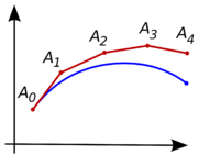
The idea is that while the curve is initially unknown, its starting point, which we denote by

is known (see the picture on top right). Then, from the differential equation, the slope to the curve at

can be computed, and so, the tangent line.

Take a small step along that tangent line up to a point

If we pretend that

is still on the curve, the same reasoning as for the point

above can be used. After several steps, a polygonal curve

is computed. In general, this curve does not diverge too far from the original unknown curve, and the error between the two curves can be made small if the step size is small enough and the interval of computation is finite (although things are more complicated for stiff equation

Stiff equation

In mathematics, a stiff equation is a differential equation for which certain numerical methods for solving the equation are numerically unstable, unless the step size is taken to be extremely small. It has proved difficult to formulate a precise definition of stiffness, but the main idea is that...

s, as discussed below).

Derivation

We want to approximate the solution of the initial value problem

by using the first two terms of the Taylor expansion of y, which represents the linear approximation around the point (t₀,y(t₀)) . One step of the Euler method from t_n to t_n+1 = t_n + h is

The Euler method is explicit, i.e. the solution

is an explicit function of

for

.

While the Euler method integrates a first order ODE, any ODE of order N can be represented as a first-order ODE:
to treat the equation

,

we introduce auxiliary variables

and obtain
the equivalent equation

This is a first-order system in the variable

and can be handled by Euler's method or, in fact, any other scheme for first-order systems.

Example

Given the differential equation

and the initial point

, we would like to use the Euler method to approximate

using step size

.

The Euler method is

so first we must compute

. This simple differential equation depends only on

, so we need only worry about inputting the values for

By doing the above step, we have found the slope of the line that is tangent to the solution curve at the point

. Recall that the slope is defined as the change in

divided by the change in

, or

.

The next step is to multiply the above value by the step size

Since the step size is the change in

, when we multiply the step size and the slope of the tangent, we get a change in

value. This value is then added to the initial

value to obtain the next value to be used for computations.

The above steps should be repeated to find

and

Due to the repetitive nature of this algorithm, it can be helpful to organize computations in a chart form, as seen below, to avoid making errors.


1	0	1	1	1	2
2	1	2	1	2	4
4	2	4	1	4	8

Error

The magnitude of the errors arising from the Euler method can be demonstrated by comparison with a Taylor expansion of y. If we assume that

and

are known exactly at a time

then the Euler method gives the approximate solution at time

as:

In comparison, the Taylor expansion in

about

gives:

Since we know that

it follows that

This, along with

can be inserted into the Taylor expansion in

about

The error introduced by the Euler method is given by the difference between these equations:

For small

, the dominant error per step, or the local truncation error

Truncation error (numerical integration)

Trunction errors in numerical integration are of two kinds:* local truncation errors – the error caused by one iteration, and* global truncation errors – the cumulative error cause by many iterations.- Definitions :...

, is proportional to

. To solve the problem over a given range of

, the number of steps needed is proportional to

so it is to be expected that the total error at the end of the fixed time, or the global truncation error, will be proportional to

(error per step times number of steps). Because the global truncation error is proportional to

, the Euler method is said to be first order. This makes the Euler method less accurate (for small

) than other higher-order techniques such as Runge-Kutta methods and linear multistep methods.

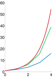
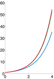
As stated in the introduction, decreasing the step size can help to make the approximation more accurate and decrease the error between the two curves. The error to three decimal places for the example in the above section (with step size

)is the following:

When the step size is changed to

our

value becomes

. The error, then, for step size

is the following:

Although the error has decreased, our approximation is still not particularly accurate. In addition, since the step size decreased with no change in the interval, the number of iterations has increased to thirty. While possible, it is no longer reasonable to do these computations by hand.

Error bound

As with other methods, there is a way for us to determine an error bound for a particular problem. The error bound on the global error is given by:

where

is the step size,

is the upper bound on the second derivative of

on the given interval (which must be estimated), and

is the Lipschitz constant

Lipschitz continuity

In mathematical analysis, Lipschitz continuity, named after Rudolf Lipschitz, is a strong form of uniform continuity for functions. Intuitively, a Lipschitz continuous function is limited in how fast it can change: for every pair of points on the graph of this function, the absolute value of the...

.

If the error bound is computed, it can be seen, once again, that if small error is desired, the step size

must be very small.

For instance, let us calculate the step size required for global truncation error to be

, assuming a maximum value for the second derivative of

, a Lipschitz constant of

, and

from zero to four. Using the equation given, we obtain the following:

which means that h must be smaller than the above to get the desired error or less, and 4/h, or about 1072 iterations will need to be completed to do so. The large number of steps, and thus high computation cost, supports the use of alternative, higher-order methods such as Runge–Kutta methods or linear multistep methods.

Numerical stability

The Euler method can also be numerically unstable

Numerical stability

In the mathematical subfield of numerical analysis, numerical stability is a desirable property of numerical algorithms. The precise definition of stability depends on the context, but it is related to the accuracy of the algorithm....

, especially for stiff equation

Stiff equation

s. This limitation—along with its slow convergence of error with h—means that the Euler method is not often used, except as a simple example of numerical integration. The instability can be avoided by using the Euler–Cromer algorithm.

External links

Euler's Method for O.D.E.'s

The source of this article is wikipedia, the free encyclopedia. The text of this article is licensed under the GFDL.

Informal geometrical description

Derivation

Example

Error

Error bound

Numerical stability

See also

External links