

On shell renormalization scheme
Encyclopedia
In quantum field theory
, and especially in quantum electrodynamics
, the interacting theory leads to infinite quantities that have to be absorbed in a renormalization
procedure, in order to be able to predict measurable quantities. The renormalization scheme can depend on the type of particles that are being considered. For particles that can travel asymptotically large distances, or for low energy processes, the on-shell scheme, also known as the physical scheme, is appropriate. If these conditions are not fulfilled, one can turn to other schemes, like the Minimal subtraction scheme
.
which are useful tools to predict, for example, the result of scattering experiments. In a theory where the only field is the Dirac field
, the Feynman propagator reads
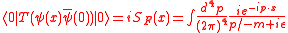
where is the time-ordering operator,
  the vacuum in the non interacting theory,
  and
and  the Dirac field and its Dirac adjoint, and where the left handside of the equation is the two-point correlation function
of the Dirac field.
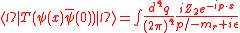
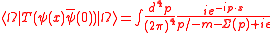
In a new theory, the Dirac field can interact with another field, for example with the electromagnetic field in quantum electrodynamics, and the strength of the interaction is measured by a parameter, in the case of QED it is the bare electron charge, . The general form of the propagator should remain unchanged, meaning that if
  now represents the vacuum in the interacting theory, the two-point correlation function would now read
Two new quantities have been introduced. First the renormalized mass has been defined as the pole in the Fourier transform of the Feynman propagator. This is the main prescription of the on-shell renormalization scheme (there is then no need to introduce other mass scales like in the minimal substraction scheme). The quantity
  represents the new strength of the Dirac field. As the interaction is turned down to zero by letting
  , these new parameters should tend to a value so as to recover the propagator of the free fermion, namely
  and
and  .
.
This means that and
and  can be defined as a serie in
  if this parameter is small enough (in the unit system where
  ,
,  , where
  is the fine-structure constant
). Thus these parameters can be expressed as


On the other hand, the modification to the propagator can be calculated up to a certain order in using Feynman diagrams. These modifications are summed up in the fermion self energy
These corrections are often divergent because they countain loops
.
By identifying the two expressions of the correlation function up to a certain order in , the counterterms can be defined, and they are going to absorb the divergent contributions of the corrections to the fermion propagator. Thus, the renormalized quantities, such as
  , will remain finite, and will be the quantities measured in experiments.
 in the interacting theory. The photon self energy is noted
  and the metric tensor
 (here taking the +--- convention)

The behaviour of the counterterm is independent of the momentum of the incoming photon
  . To fix it, the behaviour of QED at large distances (which should help recover classical electrodynamics), ie when
  , is used :
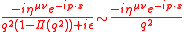
Thus the counterterm is fixed with the value of
  .
.
leads to the renormalization of the electric charge . This renormalization, and the fixing of renormalization terms is done using what is known from classical electrodynamics at large space scales. This leads to the value of the counterterm
  , which is, in fact, equal to
  because of the Ward-Takahashi identity. It is this calculation that account for the anomalous magnetic dipole moment
of fermions.
 ) that have been defined from the form of the propagator. However they can also be defined from the QED lagrangian, which will be done in this section, and these definitions are equivalent. The Lagrangian that describes the physics of quantum electrodynamics
is

where is the field strength tensor
, is the Dirac spinor (the relativistic equivalent of the wavefunction
), and A the electromagnetic four-potential
. The parameters of the theory are and
and  . These quantities happen to be infinite due to loop corrections (see below). One can define the renormalized quantities (which will be finite and observable) :

The are called counterterms (some other definitions of them are possible). They are supposed to be small in the parameter e. The Lagrangian now reads in terms of renormalized quantities (to first order in the counterterms) :

A renormalization prescription is a set of rules that describes what part of the divergences should be in the renormalized quantities and what parts should be in the counterterms. The prescription is often based on the theory of free fields, that is of the behaviour of and A when they do not interact (which corresponds to removing the term
  in the Lagrangian).
Quantum field theory
Quantum field theory provides a theoretical framework for constructing quantum mechanical models of systems classically parametrized by an infinite number of dynamical degrees of freedom, that is, fields and many-body systems. It is the natural and quantitative language of particle physics and...
, and especially in quantum electrodynamics
Quantum electrodynamics
Quantum electrodynamics is the relativistic quantum field theory of electrodynamics. In essence, it describes how light and matter interact and is the first theory where full agreement between quantum mechanics and special relativity is achieved...
, the interacting theory leads to infinite quantities that have to be absorbed in a renormalization
Renormalization
In quantum field theory, the statistical mechanics of fields, and the theory of self-similar geometric structures, renormalization is any of a collection of techniques used to treat infinities arising in calculated quantities....
procedure, in order to be able to predict measurable quantities. The renormalization scheme can depend on the type of particles that are being considered. For particles that can travel asymptotically large distances, or for low energy processes, the on-shell scheme, also known as the physical scheme, is appropriate. If these conditions are not fulfilled, one can turn to other schemes, like the Minimal subtraction scheme
Minimal subtraction scheme
In quantum field theory, the minimal subtraction scheme, or MS scheme is a particular renormalization scheme used to absorb the infinities that arise in perturbative calculations beyond leading order, introduced independently by and...
.
Fermion propagator in the interacting theory
Knowing the different propagators is the basis for being able to calculate Feynman diagramsFeynman diagram
Feynman diagrams are a pictorial representation scheme for the mathematical expressions governing the behavior of subatomic particles, first developed by the Nobel Prize-winning American physicist Richard Feynman, and first introduced in 1948...
which are useful tools to predict, for example, the result of scattering experiments. In a theory where the only field is the Dirac field
Fermionic field
In quantum field theory, a fermionic field is a quantum field whose quanta are fermions; that is, they obey Fermi-Dirac statistics. Fermionic fields obey canonical anticommutation relations rather than the canonical commutation relations of bosonic fields....
, the Feynman propagator reads
where
is the time-ordering operator, the vacuum in the non interacting theory, and the Dirac field and its Dirac adjoint, and where the left handside of the equation is the two-point correlation functionCorrelation function (quantum field theory)
In quantum field theory, the matrix element computed by inserting a product of operators between two states, usually the vacuum states, is called a correlation function....
of the Dirac field.
In a new theory, the Dirac field can interact with another field, for example with the electromagnetic field in quantum electrodynamics, and the strength of the interaction is measured by a parameter, in the case of QED it is the bare electron charge,
. The general form of the propagator should remain unchanged, meaning that if now represents the vacuum in the interacting theory, the two-point correlation function would now readTwo new quantities have been introduced. First the renormalized mass
has been defined as the pole in the Fourier transform of the Feynman propagator. This is the main prescription of the on-shell renormalization scheme (there is then no need to introduce other mass scales like in the minimal substraction scheme). The quantity represents the new strength of the Dirac field. As the interaction is turned down to zero by letting , these new parameters should tend to a value so as to recover the propagator of the free fermion, namely and .This means that
and can be defined as a serie in if this parameter is small enough (in the unit system where , , where is the fine-structure constantFine-structure constant
In physics, the fine-structure constant is a fundamental physical constant, namely the coupling constant characterizing the strength of the electromagnetic interaction. Being a dimensionless quantity, it has constant numerical value in all systems of units...
). Thus these parameters can be expressed as
On the other hand, the modification to the propagator can be calculated up to a certain order in
using Feynman diagrams. These modifications are summed up in the fermion self energy These corrections are often divergent because they countain loops
One-loop Feynman diagram
In physics, a one-loop Feynman diagram is a connected Feynman diagram with only one cycle . Such a diagram can be obtained from a connected tree diagram by taking two external lines of the same type and joining them together into an edge....
.
By identifying the two expressions of the correlation function up to a certain order in
, the counterterms can be defined, and they are going to absorb the divergent contributions of the corrections to the fermion propagator. Thus, the renormalized quantities, such as , will remain finite, and will be the quantities measured in experiments.Photon propagator
Just like what has been done with the fermion propagator, the form of the photon propagator inspired by the free photon field will be compared to the photon propagator calculated up to a certain order in in the interacting theory. The photon self energy is noted and the metric tensorMinkowski space
In physics and mathematics, Minkowski space or Minkowski spacetime is the mathematical setting in which Einstein's theory of special relativity is most conveniently formulated...
(here taking the +--- convention)The behaviour of the counterterm
is independent of the momentum of the incoming photon . To fix it, the behaviour of QED at large distances (which should help recover classical electrodynamics), ie when , is used :Thus the counterterm
is fixed with the value of .Vertex function
A similar reasoning using the vertex functionVertex function
In quantum electrodynamics, the vertex function describes the coupling between a photon and an electron beyond the leading order of perturbation theory...
leads to the renormalization of the electric charge
. This renormalization, and the fixing of renormalization terms is done using what is known from classical electrodynamics at large space scales. This leads to the value of the counterterm , which is, in fact, equal to because of the Ward-Takahashi identity. It is this calculation that account for the anomalous magnetic dipole momentAnomalous magnetic dipole moment
In quantum electrodynamics, the anomalous magnetic moment of a particle is a contribution of effects of quantum mechanics, expressed by Feynman diagrams with loops, to the magnetic moment of that particle...
of fermions.
Rescaling of the QED Lagrangian
We have considered some proportionality factors (like the) that have been defined from the form of the propagator. However they can also be defined from the QED lagrangian, which will be done in this section, and these definitions are equivalent. The Lagrangian that describes the physics of quantum electrodynamicsQuantum electrodynamics
Quantum electrodynamics is the relativistic quantum field theory of electrodynamics. In essence, it describes how light and matter interact and is the first theory where full agreement between quantum mechanics and special relativity is achieved...
is
where
is the field strength tensorElectromagnetic tensor
The electromagnetic tensor or electromagnetic field tensor is a mathematical object that describes the electromagnetic field of a physical system in Maxwell's theory of electromagnetism...
,
is the Dirac spinor (the relativistic equivalent of the wavefunctionWavefunction
Not to be confused with the related concept of the Wave equationA wave function or wavefunction is a probability amplitude in quantum mechanics describing the quantum state of a particle and how it behaves. Typically, its values are complex numbers and, for a single particle, it is a function of...
), and A the electromagnetic four-potential
Electromagnetic four-potential
The electromagnetic four-potential is a potential from which the electromagnetic field can be derived. It combines both the electric scalar potential and the magnetic vector potential into a single space-time four-vector. In a given reference frame, the first component is the scalar potential and...
. The parameters of the theory are
and . These quantities happen to be infinite due to loop corrections (see below). One can define the renormalized quantities (which will be finite and observable) :The
are called counterterms (some other definitions of them are possible). They are supposed to be small in the parameter e. The Lagrangian now reads in terms of renormalized quantities (to first order in the counterterms) :A renormalization prescription is a set of rules that describes what part of the divergences should be in the renormalized quantities and what parts should be in the counterterms. The prescription is often based on the theory of free fields, that is of the behaviour of
and A when they do not interact (which corresponds to removing the term in the Lagrangian).