
Least mean squares filter
Encyclopedia
Least mean squares algorithms are a class of adaptive filter
used to mimic a desired filter by finding the filter coefficients that relate to producing the least mean squares of the error signal (difference between the desired and the actual signal). It is a stochastic gradient descent
method in that the filter is only adapted based on the error at the current time. It was invented in 1960 by Stanford University
professor Bernard Widrow
and his first Ph.D. student, Ted Hoff.
Relationship to the least mean squares filter
The realization of the causal Wiener filter looks a lot like the solution to the least squares estimate, except in the signal processing domain. The least squares solution, for input matrix and output vector
is

The FIR Wiener filter is related to the least mean squares filter, but minimizing its error criterion does not rely on cross-correlations or auto-correlations. Its solution converges to the Wiener filter solution.
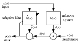
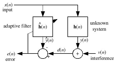
Most linear adaptive filtering problems can be formulated using the block diagram above. That is, an unknown system is to be identified and the adaptive filter attempts to adapt the filter
  to make it as close as possible to
  , while using only observable signals
  ,
,  and
and  ; but
; but  ,
,  and
and  are not directly observable. Its solution is closely related to the Wiener filter
.


 which minimize a cost function.
We start by defining the cost function as
where is the error at the current sample 'n' and
  denotes the expected value
.
This cost function ( ) is the mean square error, and it is minimized by the LMS. This is where the LMS gets its name. Applying steepest descent means to take the partial derivative
s with respect to the individual entries of the filter coefficient (weight) vector
where is the gradient
operator.

Now, is a vector which points towards the steepest ascent of the cost function. To find the minimum of the cost function we need to take a step in the opposite direction of
  . To express that in mathematical terms
where is the step size(adaptation constant). That means we have found a sequential update algorithm which minimizes the cost function. Unfortunately, this algorithm is not realizable until we know
  .
.
Generally, the expectation above is not computed. Instead, to run the LMS in an online (updating after each new sample is received) environment, we use an instantaneous estimate of that expectation. See below.
 must be approximated. This can be done with the following unbiased estimator

where indicates the number of samples we use for that estimate. The simplest case is

For that simple case the update algorithm follows as
Indeed this constitutes the update algorithm for the LMS filter.
 th order algorithm can be summarized as
where denotes the Hermitian transpose of
  .
.
 is constant, and that the input signal
  is wide-sense stationary.
Then converges to
  as
as  if and only if
where is the greatest eigenvalue of the autocorrelation
matrix . If this condition is not fulfilled, the algorithm becomes unstable and
  diverges.
Maximum convergence speed is achieved when
where is the smallest eigenvalue of
  .
.
Given that is less than or equal to this optimum, the convergence speed is determined by
  , with a larger value yielding faster convergence. This means that faster convergence can be achieved when
  is close to
  , that is, the maximum achievable convergence speed depends on the eigenvalue spread of
  .
.
A white noise
signal has autocorrelation matrix , where
  is the variance of the signal. In this case all eigenvalues are equal, and the eigenvalue spread is the minimum over all possible matrices.
The common interpretation of this result is therefore that the LMS converges quickly for white input signals, and slowly for colored input signals, such as processes with low-pass or high-pass characteristics.
It is important to note that the above upperbound on only enforces stability in the mean, but the coefficients of
  can still grow infinitely large, i.e. divergence of the coefficients is still possible. A more practical bound is
where denotes the trace of
  . This bound guarantees that the coefficients of
  do not diverge (in practice, the value of
  should not be chosen close to this upper bound, since it is somewhat optimistic due to approximations and assumptions made in the derivation of the bound).
 . This makes it very hard (if not impossible) to choose a learning rate
  that guarantees stability of the algorithm (Haykin 2002). The Normalised least mean squares filter (NLMS) is a variant of the LMS algorithm that solves this problem by normalising with the power of the input. The NLMS algorithm can be summarised as:
 ), then the optimal learning rate for the NLMS algorithm is
and is independent of the input and the real (unknown) impulse response
  . In the general case with interference (
 ), the optimal learning rate is
The results above assume that the signals and
and  are uncorrelated to each other, which is generally the case in practice.
 , we can derive the expected misalignment for the next sample as:
Let and
and 
Assuming independence, we have:
The optimal learning rate is found at , which leads to:
Adaptive filter
An adaptive filter is a filter that self-adjusts its transfer function according to an optimization algorithm driven by an error signal. Because of the complexity of the optimization algorithms, most adaptive filters are digital filters. By way of contrast, a non-adaptive filter has a static...
used to mimic a desired filter by finding the filter coefficients that relate to producing the least mean squares of the error signal (difference between the desired and the actual signal). It is a stochastic gradient descent
Stochastic gradient descent
Stochastic gradient descent is an optimization method for minimizing an objective function that is written as a sum of differentiable functions.- Background :...
method in that the filter is only adapted based on the error at the current time. It was invented in 1960 by Stanford University
Stanford University
The Leland Stanford Junior University, commonly referred to as Stanford University or Stanford, is a private research university on an campus located near Palo Alto, California. It is situated in the northwestern Santa Clara Valley on the San Francisco Peninsula, approximately northwest of San...
professor Bernard Widrow
Bernard Widrow
Bernard Widrow is a U.S. professor of electrical engineering at Stanford University. He is the co-inventor of the Widrow–Hoff least mean squares filter adaptive algorithm with his then doctoral student Ted Hoff...
and his first Ph.D. student, Ted Hoff.
Problem formulation
Relationship to the least mean squares filter
The realization of the causal Wiener filter looks a lot like the solution to the least squares estimate, except in the signal processing domain. The least squares solution, for input matrix
and output vector is
The FIR Wiener filter is related to the least mean squares filter, but minimizing its error criterion does not rely on cross-correlations or auto-correlations. Its solution converges to the Wiener filter solution.
Most linear adaptive filtering problems can be formulated using the block diagram above. That is, an unknown system
is to be identified and the adaptive filter attempts to adapt the filter to make it as close as possible to , while using only observable signals , and ; but , and are not directly observable. Its solution is closely related to the Wiener filterWiener filter
In signal processing, the Wiener filter is a filter proposed by Norbert Wiener during the 1940s and published in 1949. Its purpose is to reduce the amount of noise present in a signal by comparison with an estimation of the desired noiseless signal. The discrete-time equivalent of Wiener's work was...
.
definition of symbols
Idea
The idea behind LMS filters is to use steepest descent to find filter weights which minimize a cost function.We start by defining the cost function as
where
is the error at the current sample 'n' and denotes the expected valueExpected value
In probability theory, the expected value of a random variable is the weighted average of all possible values that this random variable can take on...
.
This cost function (
) is the mean square error, and it is minimized by the LMS. This is where the LMS gets its name. Applying steepest descent means to take the partial derivativePartial derivative
In mathematics, a partial derivative of a function of several variables is its derivative with respect to one of those variables, with the others held constant...
s with respect to the individual entries of the filter coefficient (weight) vector
where
is the gradientGradient
In vector calculus, the gradient of a scalar field is a vector field that points in the direction of the greatest rate of increase of the scalar field, and whose magnitude is the greatest rate of change....
operator.
Now,
is a vector which points towards the steepest ascent of the cost function. To find the minimum of the cost function we need to take a step in the opposite direction of . To express that in mathematical termswhere
is the step size(adaptation constant). That means we have found a sequential update algorithm which minimizes the cost function. Unfortunately, this algorithm is not realizable until we know .Generally, the expectation above is not computed. Instead, to run the LMS in an online (updating after each new sample is received) environment, we use an instantaneous estimate of that expectation. See below.
Simplifications
For most systems the expectation function must be approximated. This can be done with the following unbiased estimatorEstimator
In statistics, an estimator is a rule for calculating an estimate of a given quantity based on observed data: thus the rule and its result are distinguished....
where
indicates the number of samples we use for that estimate. The simplest case is For that simple case the update algorithm follows as
Indeed this constitutes the update algorithm for the LMS filter.
LMS algorithm summary
The LMS algorithm for ath order algorithm can be summarized as
| Parameters: |  filter order filter order |
 step size step size |
|
| Initialisation: |  |
| Computation: | For  |
| |
|
| |
|
| |
where
denotes the Hermitian transpose of .Convergence and stability in the mean
Assume that the true filter is constant, and that the input signal is wide-sense stationary.Then
converges to as if and only ifwhere
is the greatest eigenvalue of the autocorrelationAutocorrelation
Autocorrelation is the cross-correlation of a signal with itself. Informally, it is the similarity between observations as a function of the time separation between them...
matrix
. If this condition is not fulfilled, the algorithm becomes unstable and diverges.Maximum convergence speed is achieved when
where
is the smallest eigenvalue of .Given that
is less than or equal to this optimum, the convergence speed is determined by , with a larger value yielding faster convergence. This means that faster convergence can be achieved when is close to , that is, the maximum achievable convergence speed depends on the eigenvalue spread of .A white noise
White noise
White noise is a random signal with a flat power spectral density. In other words, the signal contains equal power within a fixed bandwidth at any center frequency...
signal has autocorrelation matrix
, where is the variance of the signal. In this case all eigenvalues are equal, and the eigenvalue spread is the minimum over all possible matrices.The common interpretation of this result is therefore that the LMS converges quickly for white input signals, and slowly for colored input signals, such as processes with low-pass or high-pass characteristics.
It is important to note that the above upperbound on
only enforces stability in the mean, but the coefficients of can still grow infinitely large, i.e. divergence of the coefficients is still possible. A more practical bound iswhere
denotes the trace of . This bound guarantees that the coefficients of do not diverge (in practice, the value of should not be chosen close to this upper bound, since it is somewhat optimistic due to approximations and assumptions made in the derivation of the bound).Normalised least mean squares filter (NLMS)
The main drawback of the "pure" LMS algorithm is that it is sensitive to the scaling of its input. This makes it very hard (if not impossible) to choose a learning rate that guarantees stability of the algorithm (Haykin 2002). The Normalised least mean squares filter (NLMS) is a variant of the LMS algorithm that solves this problem by normalising with the power of the input. The NLMS algorithm can be summarised as:| Parameters: |  filter order filter order |
 step size step size |
|
| Initialization: |  |
| Computation: | For  |
| |
|
| |
|
| |
Optimal learning rate
It can be shown that if there is no interference (), then the optimal learning rate for the NLMS algorithm isand is independent of the input
and the real (unknown) impulse response . In the general case with interference (), the optimal learning rate isThe results above assume that the signals
and are uncorrelated to each other, which is generally the case in practice.Proof
Let the filter misalignment be defined as, we can derive the expected misalignment for the next sample as:


Let
and 

Assuming independence, we have:


The optimal learning rate is found at
, which leads to:


See also
- Recursive least squares
- For statistical techniques relevant to LMS filter see Least squaresLeast squaresThe method of least squares is a standard approach to the approximate solution of overdetermined systems, i.e., sets of equations in which there are more equations than unknowns. "Least squares" means that the overall solution minimizes the sum of the squares of the errors made in solving every...
. - Similarities between Wiener and LMSSimilarities between Wiener and LMSThe Least mean squares filter solution converges to the Wiener filter solution, assuming that the unknown system is LTI and the noise is stationary. Both filters can be used to identify the impulse response of an unknown system, knowing only the original input signal and the output of the unknown...
- Multidelay block frequency domain adaptive filterMultidelay block frequency domain adaptive filterThe Multidelay block frequency domain adaptive filter algorithm is a block-based frequency domain implementation of the Least mean squares filter algorithm.- Introduction :...
- Kernel adaptive filterKernel adaptive filterKernel adaptive filtering is an adaptive filtering technique for general nonlinear problems. It is a natural generalization of linear adaptive filtering in reproducing kernel Hilbert spaces. Kernel adaptive filters are online kernel methods, closely related to some artificial neural networks such...
External links
- LMS Algorithm in Adaptive Antenna Arrays www.antenna-theory.com
- LMS Noise cancellation demo www.advsolned.com