
Illustration of the central limit theorem
Encyclopedia
This article gives two concrete illustrations of the central limit theorem
. Both involve the sum of independent and identically-distributed random variables and show how the probability distribution
of the sum approaches the normal distribution as the number of terms in the sum increases.
The first illustration involves a continuous probability distribution, for which the random variables have a probability density function
.
The second illustration, for which most of the computation can be done by hand, involves a discrete probability distribution, which is characterized by a probability mass function
.
A free full-featured interactive simulation that allows the user to set up various distributions and adjust the sampling parameters is available through the External links section at the bottom of this page.
of the density functions of the original variables.
Thus, the density of the sum of m+n terms of a sequence of independent identically distributed variables equals the convolution of the densities of the sums of m terms and of n term. In particular, the density of the sum of n+1 terms equals the convolution of the density of the sum of n terms with the original density (the "sum" of 1 term).
A probability density function
is shown in the first figure below. Then the densities of the sums of two, three, and four independent identically distributed variables, each having the original density, are shown in the following figures.
If the original density is a piecewise
polynomial
, as it is in the example, then so are the sum densities, of increasingly higher degree. Although the original density is far from normal, the density of the sum of just a few variables with that density is much smoother and has some of the qualitative features of the normal density.
The convolutions were computed via the discrete Fourier transform
. A list of values y = f(x0 + k Δx) was constructed, where f is the original density function, and Δx is approximately equal to 0.002, and k is equal to 0 through 1000. The discrete Fourier transform Y of y was computed. Then the convolution of f with itself is proportional to the inverse discrete Fourier transform of the pointwise product
of Y with itself.
4545
The density of the sum is the convolution of the above density with itself.
The sum of two variables has mean 0.
The density shown in the figure at right has been rescaled by √2, so that its standard deviation is 1.
This density is already smoother than the original.
There are obvious lumps, which correspond to the intervals on which the original density was defined.
The density of the sum is the convolution of the first density with the second.
The sum of three variables has mean 0.
The density shown in the figure at right has been rescaled by √3, so that its standard deviation is 1.
This density is even smoother than the preceding one.
The lumps can hardly be detected in this figure.
The density of the sum is the convolution of the first density with the third.
The sum of four variables has mean 0.
The density shown in the figure at right has been rescaled by √4, so that its standard deviation is 1.
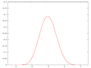
This density appears qualitatively very similar to a normal density.
No lumps can be distinguished by the eye.

The probability mass function of the random variable X may be depicted by the following bar graph:
o o o
-------------
1 2 3
Clearly this looks nothing like the bell-shaped curve of the normal distribution. Contrast the above with the depictions below.

The probability mass function of this sum may be depicted thus:
o
o o o
o o o o o
----------------------------
2 3 4 5 6
This still does not look very much like the bell-shaped curve, but, like the bell-shaped curve and unlike the probability mass function of X itself, it is higher in the middle than in the two tails.

The probability mass function of this sum may be depicted thus:
o
o o o
o o o
o o o
o o o o o
o o o o o
o o o o o o o
---------------------------------
3 4 5 6 7 8 9
Not only is this bigger at the center than it is at the tails, but as one moves toward the center from either tail, the slope first increases and then decreases, just as with the bell-shaped curve.
The degree of its resemblance to the bell-shaped curve can be quantified as follows. Consider
How close is this to what a normal approximation would give? It can readily be seen that the expected value of Y = X1 + X2 + X3 is 6 and the standard deviation of Y is the square root of 2. Since Y ≤ 7 (weak inequality) if and only if Y < 8 (strict inequality), we use a continuity correction
and seek

where Z has a standard normal distribution. The difference between 0.85185... and 0.85558... seems remarkably small when it is considered that the number of independent random variables that were added was only three.
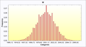 The following image shows the result of a simulation based on the example presented in this page. The extraction from the uniform distribution is repeated 1,000 times, and the results are summed.
Since the simulation is based on the Monte Carlo method
, the process is repeated 10,000 times. The results shows that the distribution of the sum of 1,000 uniform extractions resembles the bell-shaped curve very well.
Central limit theorem
In probability theory, the central limit theorem states conditions under which the mean of a sufficiently large number of independent random variables, each with finite mean and variance, will be approximately normally distributed. The central limit theorem has a number of variants. In its common...
. Both involve the sum of independent and identically-distributed random variables and show how the probability distribution
Probability distribution
In probability theory, a probability mass, probability density, or probability distribution is a function that describes the probability of a random variable taking certain values....
of the sum approaches the normal distribution as the number of terms in the sum increases.
The first illustration involves a continuous probability distribution, for which the random variables have a probability density function
Probability density function
In probability theory, a probability density function , or density of a continuous random variable is a function that describes the relative likelihood for this random variable to occur at a given point. The probability for the random variable to fall within a particular region is given by the...
.
The second illustration, for which most of the computation can be done by hand, involves a discrete probability distribution, which is characterized by a probability mass function
Probability mass function
In probability theory and statistics, a probability mass function is a function that gives the probability that a discrete random variable is exactly equal to some value...
.
A free full-featured interactive simulation that allows the user to set up various distributions and adjust the sampling parameters is available through the External links section at the bottom of this page.
Illustration of the continuous case
The density of the sum of two independent real-valued random variables equals the convolutionConvolution
In mathematics and, in particular, functional analysis, convolution is a mathematical operation on two functions f and g, producing a third function that is typically viewed as a modified version of one of the original functions. Convolution is similar to cross-correlation...
of the density functions of the original variables.
Thus, the density of the sum of m+n terms of a sequence of independent identically distributed variables equals the convolution of the densities of the sums of m terms and of n term. In particular, the density of the sum of n+1 terms equals the convolution of the density of the sum of n terms with the original density (the "sum" of 1 term).
A probability density function
Probability density function
In probability theory, a probability density function , or density of a continuous random variable is a function that describes the relative likelihood for this random variable to occur at a given point. The probability for the random variable to fall within a particular region is given by the...
is shown in the first figure below. Then the densities of the sums of two, three, and four independent identically distributed variables, each having the original density, are shown in the following figures.
If the original density is a piecewise
Piecewise
On mathematics, a piecewise-defined function is a function whose definition changes depending on the value of the independent variable...
polynomial
Polynomial
In mathematics, a polynomial is an expression of finite length constructed from variables and constants, using only the operations of addition, subtraction, multiplication, and non-negative integer exponents...
, as it is in the example, then so are the sum densities, of increasingly higher degree. Although the original density is far from normal, the density of the sum of just a few variables with that density is much smoother and has some of the qualitative features of the normal density.
The convolutions were computed via the discrete Fourier transform
Discrete Fourier transform
In mathematics, the discrete Fourier transform is a specific kind of discrete transform, used in Fourier analysis. It transforms one function into another, which is called the frequency domain representation, or simply the DFT, of the original function...
. A list of values y = f(x0 + k Δx) was constructed, where f is the original density function, and Δx is approximately equal to 0.002, and k is equal to 0 through 1000. The discrete Fourier transform Y of y was computed. Then the convolution of f with itself is proportional to the inverse discrete Fourier transform of the pointwise product
Pointwise product
The pointwise product of two functions is another function, obtained by multiplying the image of the two functions at each value in the domain...
of Y with itself.
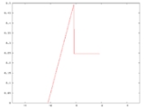
Original probability density function
We start with a probability density function. This function, although discontinuous, is far from the most pathological example that could be created. It is a piecewise polynomial, with pieces of degrees 0 and 1. The mean of this distribution is 0 and its standard deviation is 1.4545
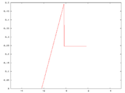
Probability density function of the sum of two terms
Next we compute the density of the sum of two independent variables, each having the above density.The density of the sum is the convolution of the above density with itself.
The sum of two variables has mean 0.
The density shown in the figure at right has been rescaled by √2, so that its standard deviation is 1.
This density is already smoother than the original.
There are obvious lumps, which correspond to the intervals on which the original density was defined.
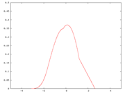
Probability density function of the sum of three terms
We then compute the density of the sum of three independent variables, each having the above density.The density of the sum is the convolution of the first density with the second.
The sum of three variables has mean 0.
The density shown in the figure at right has been rescaled by √3, so that its standard deviation is 1.
This density is even smoother than the preceding one.
The lumps can hardly be detected in this figure.
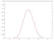
Probability density function of the sum of four terms
Finally, we compute the density of the sum of four independent variables, each having the above density.The density of the sum is the convolution of the first density with the third.
The sum of four variables has mean 0.
The density shown in the figure at right has been rescaled by √4, so that its standard deviation is 1.
This density appears qualitatively very similar to a normal density.
No lumps can be distinguished by the eye.
Illustration of the discrete case
This section illustrates the central limit theorem via an example for which the computation can be done quickly by hand on paper, unlike the more computing-intensive example of the previous section.Original probability mass function
Suppose the probability distribution of a discrete random variable X puts equal weights on 1, 2, and 3:The probability mass function of the random variable X may be depicted by the following bar graph:
o o o
-------------
1 2 3
Clearly this looks nothing like the bell-shaped curve of the normal distribution. Contrast the above with the depictions below.
Probability mass function of the sum of two terms
Now consider the sum of two independent copies of X:The probability mass function of this sum may be depicted thus:
o
o o o
o o o o o
----------------------------
2 3 4 5 6
This still does not look very much like the bell-shaped curve, but, like the bell-shaped curve and unlike the probability mass function of X itself, it is higher in the middle than in the two tails.
Probability mass function of the sum of three terms
Now consider the sum of three independent copies of this random variable:The probability mass function of this sum may be depicted thus:
o
o o o
o o o
o o o
o o o o o
o o o o o
o o o o o o o
---------------------------------
3 4 5 6 7 8 9
Not only is this bigger at the center than it is at the tails, but as one moves toward the center from either tail, the slope first increases and then decreases, just as with the bell-shaped curve.
The degree of its resemblance to the bell-shaped curve can be quantified as follows. Consider
- Pr(X1 + X2 + X3 ≤ 7) = 1/27 + 3/27 + 6/27 + 7/27 + 6/27 = 23/27 = 0.85185... .
How close is this to what a normal approximation would give? It can readily be seen that the expected value of Y = X1 + X2 + X3 is 6 and the standard deviation of Y is the square root of 2. Since Y ≤ 7 (weak inequality) if and only if Y < 8 (strict inequality), we use a continuity correction
Continuity correction
In probability theory, if a random variable X has a binomial distribution with parameters n and p, i.e., X is distributed as the number of "successes" in n independent Bernoulli trials with probability p of success on each trial, then...
and seek
where Z has a standard normal distribution. The difference between 0.85185... and 0.85558... seems remarkably small when it is considered that the number of independent random variables that were added was only three.
Probability mass function of the sum of 1,000 terms
Since the simulation is based on the Monte Carlo method
Monte Carlo method
Monte Carlo methods are a class of computational algorithms that rely on repeated random sampling to compute their results. Monte Carlo methods are often used in computer simulations of physical and mathematical systems...
, the process is repeated 10,000 times. The results shows that the distribution of the sum of 1,000 uniform extractions resembles the bell-shaped curve very well.
External links
- Animated examples of the CLT
- General Dynamic SOCR CLT Activity
- Interactive Simulation of the Central Limit Theorem for Windows
- Java applet demonstrating the Central Limit Theorem with rolls of dice
- The SOCR CLT activity provides hands-on demonstration of the theory and applications of this limit theorem.