
Central limit theorem
Overview
Probability theory
Probability theory is the branch of mathematics concerned with analysis of random phenomena. The central objects of probability theory are random variables, stochastic processes, and events: mathematical abstractions of non-deterministic events or measured quantities that may either be single...
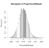
, the central limit theorem (CLT) states conditions under which the mean of a sufficiently large number of independent
Statistical independence
In probability theory, to say that two events are independent intuitively means that the occurrence of one event makes it neither more nor less probable that the other occurs...
random variables, each with finite mean and variance, will be approximately normally distributed. The central limit theorem has a number of variants. In its common form, the random variables must be identically distributed.
Unanswered Questions