

Euler–Lotka equation
Encyclopedia
The field of mathematical demography
was largely developed by Alfred J. Lotka
in the early 20th century, building on the earlier work of Leonhard Euler
. The Euler–Lotka equation, derived and discussed below, is often attributed to either of its origins – Euler, who derived a special form in 1760, or Lotka, who derived a more general continuous version.
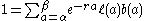
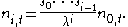
The equation in discrete time is given by
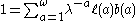
Where is the discrete growth rate, ℓ(a), is the fraction of individuals surviving to age a and b(a) is the number of individuals born at time a. The sum is taken over the entire life span of the organism.
Let B(t) be the number of births per unit time. Also define the scale factor ℓ(a), the fraction of individuals surviving to age a. Finally define b(a) to be the number of individuals born in the time step containing a.
All of these quantities can be viewed in the continuous
limit, producing the following integral expression for B:
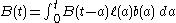
The integrand gives the number of births a years in the past multiplied by the number of offspring each of these births can produce. We integrate over all possible years to find the total rate of births at time t. We are in effect finding the contributions of all individuals of age up to t. We need not consider individuals born before the start of this analysis since we can just set the base point low enough to incorporate all of them.
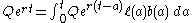
Let us then guess an exponential
solution of the form B(t) = Qert. Plugging this into the integral equation gives:
or
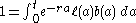
This can be rewritten in the discrete
case by turning the integral into a sum producing
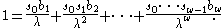
letting and
and  be the boundary ages for reproduction or defining the discrete growth rate λ = er we obtain the discrete time equation derived above:

where is the maximum age, we can extend these ages since b(a) vanishes beyond the boundaries.
as: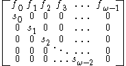
Where and
and  are survival to the next age class and per capita fecundity respectively.
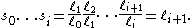
Note that where ℓ i is the probability of surviving to age
  , and
, and
 , the number of births at age
  weighted by the probability of surviving to age
  .
.
Now if we have stable growth the growth of the system is an eigenvalue of the matrix since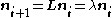 . Therefore we can use this relationship row by row to derive expressions for
  in terms of the values in the matrix and
  .
.
Introducing notation the population in age class
  at time
  , we have
  . However also
  . This implies that

By the same argument we find that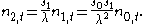
Continuing inductively
we conclude that generally
Considering the top row, we get

Now we may substitute our previous work for the terms and obtain:

First substitute the definition of the per-capita fertility and divide through by the left hand side:
Now we note the following simplification. Since we note that
This sum collapses to:

Which is the desired result.
of the Leslie matrix. We can analyze its solutions to find information about the eigenvalues of the Leslie matrix (which has implications for the stability of populations).
Considering the continuous expression f as a function of r, we can examine its roots. We notice that at negative infinity the function grows to positive infinity and at positive infinity the function approaches 0.
The first derivative
is clearly −af and the second derivative is a2f. This function is then decreasing, concave up and takes on all positive values. It is also continuous by construction so by the intermediate value theorem, it crosses r = 1 exactly once. Therefore there is exactly one real solution, which is therefore the dominant eigenvalue of the matrix the equilibrium growth rate.
This same derivation applies to the discrete case.
Demography
Demography is the statistical study of human population. It can be a very general science that can be applied to any kind of dynamic human population, that is, one that changes over time or space...
was largely developed by Alfred J. Lotka
Alfred J. Lotka
Alfred James Lotka was a US mathematician, physical chemist, and statistician, famous for his work in population dynamics and energetics. An American biophysicist best known for his proposal of the predator-prey model, developed simultaneously but independently of Vito Volterra...
in the early 20th century, building on the earlier work of Leonhard Euler
Leonhard Euler
Leonhard Euler was a pioneering Swiss mathematician and physicist. He made important discoveries in fields as diverse as infinitesimal calculus and graph theory. He also introduced much of the modern mathematical terminology and notation, particularly for mathematical analysis, such as the notion...
. The Euler–Lotka equation, derived and discussed below, is often attributed to either of its origins – Euler, who derived a special form in 1760, or Lotka, who derived a more general continuous version.
The equation in discrete time is given by
Where
is the discrete growth rate, ℓ(a), is the fraction of individuals surviving to age a and b(a) is the number of individuals born at time a. The sum is taken over the entire life span of the organism.Lotka's continuous model
A.J. Lotka in 1911 developed a continuous model of population dynamics as follows. This model tracks only the females in the population.Let B(t) be the number of births per unit time. Also define the scale factor ℓ(a), the fraction of individuals surviving to age a. Finally define b(a) to be the number of individuals born in the time step containing a.
All of these quantities can be viewed in the continuous
Continuous function
In mathematics, a continuous function is a function for which, intuitively, "small" changes in the input result in "small" changes in the output. Otherwise, a function is said to be "discontinuous". A continuous function with a continuous inverse function is called "bicontinuous".Continuity of...
limit, producing the following integral expression for B:
The integrand gives the number of births a years in the past multiplied by the number of offspring each of these births can produce. We integrate over all possible years to find the total rate of births at time t. We are in effect finding the contributions of all individuals of age up to t. We need not consider individuals born before the start of this analysis since we can just set the base point low enough to incorporate all of them.
Let us then guess an exponential
Exponential function
In mathematics, the exponential function is the function ex, where e is the number such that the function ex is its own derivative. The exponential function is used to model a relationship in which a constant change in the independent variable gives the same proportional change In mathematics,...
solution of the form B(t) = Qert. Plugging this into the integral equation gives:
or
This can be rewritten in the discrete
Discrete mathematics
Discrete mathematics is the study of mathematical structures that are fundamentally discrete rather than continuous. In contrast to real numbers that have the property of varying "smoothly", the objects studied in discrete mathematics – such as integers, graphs, and statements in logic – do not...
case by turning the integral into a sum producing
letting
and be the boundary ages for reproduction or defining the discrete growth rate λ = er we obtain the discrete time equation derived above:where
is the maximum age, we can extend these ages since b(a) vanishes beyond the boundaries.From the Leslie matrix
Let us write the Leslie matrixLeslie matrix
In applied mathematics, the Leslie matrix is a discrete, age-structured model of population growth that is very popular in population ecology. It was invented by and named after Patrick H. Leslie...
as:
Where
and are survival to the next age class and per capita fecundity respectively.Note that
where ℓ i is the probability of surviving to age , and, the number of births at age weighted by the probability of surviving to age .Now if we have stable growth the growth of the system is an eigenvalue of the matrix since
. Therefore we can use this relationship row by row to derive expressions for in terms of the values in the matrix and .Introducing notation
the population in age class at time , we have . However also . This implies thatBy the same argument we find that
Continuing inductively
Mathematical induction
Mathematical induction is a method of mathematical proof typically used to establish that a given statement is true of all natural numbers...
we conclude that generally
Considering the top row, we get
Now we may substitute our previous work for the
terms and obtain:First substitute the definition of the per-capita fertility and divide through by the left hand side:
Now we note the following simplification. Since
we note thatThis sum collapses to:
Which is the desired result.
Analysis of expression
From the above analysis we see that the Euler–Lotka equation is in fact the characteristic polynomialCharacteristic polynomial
In linear algebra, one associates a polynomial to every square matrix: its characteristic polynomial. This polynomial encodes several important properties of the matrix, most notably its eigenvalues, its determinant and its trace....
of the Leslie matrix. We can analyze its solutions to find information about the eigenvalues of the Leslie matrix (which has implications for the stability of populations).
Considering the continuous expression f as a function of r, we can examine its roots. We notice that at negative infinity the function grows to positive infinity and at positive infinity the function approaches 0.
The first derivative
Derivative
In calculus, a branch of mathematics, the derivative is a measure of how a function changes as its input changes. Loosely speaking, a derivative can be thought of as how much one quantity is changing in response to changes in some other quantity; for example, the derivative of the position of a...
is clearly −af and the second derivative is a2f. This function is then decreasing, concave up and takes on all positive values. It is also continuous by construction so by the intermediate value theorem, it crosses r = 1 exactly once. Therefore there is exactly one real solution, which is therefore the dominant eigenvalue of the matrix the equilibrium growth rate.
This same derivation applies to the discrete case.