

Dirac bracket
Encyclopedia
The Dirac bracket is a generalization of the Poisson bracket
developed by Paul Dirac
to correctly treat systems with second class constraints
in Hamiltonian mechanics
and canonical quantization
. It is an important part of Dirac's development of Hamiltonian mechanics
to handle more general Lagrangian
s. More abstractly the two form implied from the Dirac bracket is the restriction of the symplectic form
to the constraint surface in phase space
.
This article assumes familiarity with the standard Lagrangian
and Hamiltonian
formalisms, and their connection to canonical quantization
. The details of Dirac's modified Hamiltonian formalism are summarized to put the Dirac bracket in context.
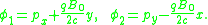
is a particle with charge and mass
  fixed in the
  -
- plane with a strong constant, homogeneous magnetic field pointing in the
  -direction with strength
  . The Lagrangian for the system with an appropriate choice of parameters is
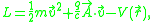
where is the vector potential
for the magnetic field, ;
;  is the speed of light in vacuum; and
  is an arbitrary external scalar potential. We use
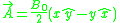
as our vector potential. Here, the hats indicate unit vectors. Later in the article they are used to distinguish quantum mechanical operators from their classical analogs. The usage should be clear from the context.
Explicitly, the Lagrangian
becomes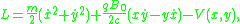
which leads to the equations of motion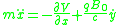
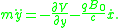
Now consider the limit where which corresponds to a very large magnetic field. In which case, one can drop the mass term to find an approximate Lagrangian
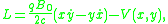
and first order equations of motion

Notice that this approximate Lagrangian is linear in the velocities which is one of the conditions under which the standard Hamiltonian procedure breaks down. While this example has been motivated as an approximation, the Lagrangian under consideration is perfectly allowable and leads to consistent equations of motion in the Lagrangian formalism.
Following the Hamiltonian procedure, the canonical momenta associated with the coordinates are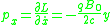
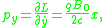
which are unusual in that they are not invertible to the velocities. A Legendre transformation
produces the Hamiltonian,
Note that this "naive" Hamiltonian has no dependence on the momenta, which means that equations of motion from Hamilton's equations are inconsistent; the Hamiltonian procedure has broken down. One might try to fix the problem by sometimes expressing the coordinates as momenta and sometimes as coordinates; however, this is neither a general nor rigorous solution. This last comment gets at the heart of the matter, that the definition of the canonical momenta implies a constraint on phase space (between momenta and coordinates) that was never taken into account.
, then one generally adds Lagrange multipliers
to the Lagrangian to account for them. The extra terms vanish when the constraints are satisfied, thereby forcing the path of stationary action to be on the constraint surface. In this case, going to the Hamiltonian formalism introduces a constraint on phase space in Hamiltonian mechanics, but the solution is similar.
Before proceeding, it is useful to understand the notions of weak equality and strong equality. Two functions on phase space, and
and  , are weakly equal if they are equal when the equations of motion are satisfied or on shell
, denoted . If
. If  and
and  are equal on and off shell, then they are called strongly equal, written
  . It is important to note that in order to get the right answer no weak equations may be used before evaluating derivatives or Poisson brackets.
The new procedure works as follows, start with a Lagrangian and define the canonical momenta in the usual way. Some of those definitions may not be invertible and instead give a constraint in phase space (as above). Constraints derived in this way or imposed from the beginning of the problem are called primary constraints. The constraints, labeled , must weakly vanish,
  .
.
Next, one finds the naive Hamiltonian, , in the usual way via a Legendre transformation, exactly as in the above example. Note that the Hamiltonian can always be written as a function of
  's and
  's only, even if the velocities cannot be inverted into functions of the momenta.
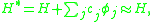
where the are not constants but functions of the coordinates and momenta. Since this new Hamiltonian is the most general function of coordinates and momenta weakly equal to the naive Hamiltonian,
  is the broadest generalization of the Hamiltonian possible.
To illuminate the more, consider how one gets the equations of motion from the naive Hamiltonian in the standard procedure. One expands the variation of the Hamiltonian out in two ways and sets them equal (using a somewhat abbreviated notation with suppressed indices and sums):
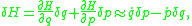
where the second equality holds after simplifying with the Euler-Lagrange equations of motion and the definition of canonical momentum. From this equality, one deduces the equations of motion in the Hamiltonian formalism from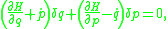
where the weak equality symbol is no longer displayed explicitly, since by definition the equations of motion only hold weakly. In the present context, one cannot simply set the coefficients of and
and  separately to zero, since the variations are somewhat restricted by the constraints. In particular, the variations must be tangent to the constraint surface.
One can demonstrate the solution to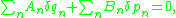
for the variations and
and  restricted by the constraints
  (assuming the constraints satisfy some regularity conditions) is generally
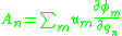
where the are arbitrary functions.
Using this result, the equations of motion become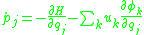

where the are functions of coordinates and velocities that can be determined, in principle, from the second equation of motion above. The Legendre transform between the Lagrangian formalism and the Hamiltonian formalism is saved at the cost of adding new variables.
 is some function of the coordinates and momenta then
if one assumes that the Poisson bracket with the (functions of the velocity) exist; this causes no problems since the contribution weakly vanishes. Now, there are some consistency conditions which must be satisfied in order for this formalism to make sense. If the constraints are going to be satisfied, then their equations of motion must weakly vanish, that is, we require
There are four different types of conditions that can result from the above:
The first case indicates that the starting Lagrangian gives inconsistent equations of motion, such as . The second case does not contribute anything new.
The third case gives new constraints in phase space. A constraint derived in this manner is called a secondary constraint. Upon finding the secondary constraint one should add it to the extended Hamiltonian and check the new consistency conditions, which may result in still more constraints. Iterate this process until there are no more constraints. The distinction between primary and secondary constraints is largely an artificial one (i.e. a constraint for the same system can be primary or secondary depending on the Lagrangian), so this article does not distinguish between them from here on. Assuming the consistency condition has been iterated until all of the constraints have been found, then will index all of them. Note this article uses secondary constraint to mean any constraint that was not initially in the problem or derived from the definition of canonical momenta; some authors distinguish between secondary constraints, tertiary constraints, et cetera.
Finally, the last case helps fix the . If, at the end of this process, the
  are not completely determined then that means there are unphysical (gauge) degrees of freedom in the system. Once all of the constraints (primary and secondary) are added to the naive Hamiltonian and the solutions to the consistency conditions for the
  are plugged in the result is called the total Hamiltonian.
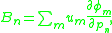
Fixing the
The  must solve a set of inhomogeneous linear equations of the form
The above equation must possess at least one solution, since otherwise the initial Lagrangian is inconsistent; however, in systems with gauge degrees of freedom, the solution will not be unique. The most general solution is of the form
where is a particular solution and
  is the most general solution to the homogeneous equation
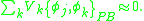
The most general solution will be a linear combination of linearly independent solutions to the above homogeneous equation. The number of linearly independent solutions equals the number of (which is the same as the number of constraints) minus the number of consistency conditions of the fourth type (in previous subsection). This is the number of unphysical degrees of freedom in the system. Labeling the linear independent solutions
  where the index
  runs from 1 to the number of unphysical degrees of freedom, the general solution to the consistency conditions is of the form
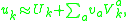
where the are completely arbitrary functions of time. A different choice of the
  corresponds to a gauge transformation and should leave the physical state of the system unchanged.

and what is denoted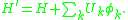
The time evolution of a function on the phase space, is governed by
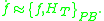
Later, the extended Hamiltonian is introduced. For gauge-invariant (physically measurable quantities) quantities all of the Hamiltonians should give the same time evolution since they are all weakly equivalent. It is only for nongauge-invariant quantities that the distinction becomes important.
Before defining Dirac brackets, first class and second class constraints need to be introduced. We call a function of coordinates and momenta first class if its Poisson bracket with all of the constraints weakly vanishes, that is,
for all . Note that the only quantities that weakly vanish are the constraints
  , and therefore anything that weakly vanishes must be strongly equal to a linear combination of the constraints. One can demonstrate that the Poisson bracket of two first class quantities must also be first class. The first class constraints are intimately connected with the unphysical degrees of freedom mentioned earlier. Namely, the number of independent first class constraints is equal to the number of unphysical degrees of freedom, and furthermore the primary first class constraints generate gauge transformations. Dirac further postulated that all secondary first class constraints are generators of gauge transformations, which turns out to be false; however, typically one operates under the assumption that all first class constraints generate gauge transformations when using this treatment.
When the first class secondary constraints are added into the Hamiltonian with arbitrary as the first class primary constraints are added to arrive at the total Hamiltonian, then one obtains the extended Hamiltonian. The extended Hamiltonian gives the most general possible time evolution for any gauge-dependent quantities, and may actually generalize the equations of motion from those of the Lagrangian formalism.
For the purposes of introducing the Dirac bracket, of more immediate interest are the second class constraints. Second class constraints are constraints that have nonvanishing Poisson bracket with at least one other constraint. For instance, consider constraints and
and  whose Poisson bracket is simply a constant,
  ,
,
Now, suppose one wishes to employ canonical quantization, then the phase space coordinates become operators whose commutators become times their classical Poisson bracket. Assuming there are no ordering issues that give rise to new quantum corrections, this implies that
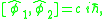
where the hats emphasize the fact that the constraints are operators. On the one hand, canonical quantization gives the above commutation relation, but on the other hand and
and  are constraints that must vanish on physical states, whereas the right hand side cannot vanish. This example illustrates the need for a generalization of the Poisson bracket that respects the system's constraints, and leads to a consistent quantization procedure.
The new bracket should be bilinear, antisymmetric, satisfy the Jacobi identity as does the Poisson bracket, reduce to the Poisson bracket for unconstrained systems, and additionally the bracket of any constraint with any other quantity must vanish. At this point, the second class constraints will be labeled . Define a matrix with entries
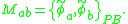
In which case, the Dirac bracket of two functions on phase space, and
and  , is defined as
where denotes the
  entry of
  's inverse matrix. Dirac proved that
  will always be invertible. It is straightforward to check that the above definition of the Dirac bracket satisfies all of the desired properties. When using canonical quantization with a constrained Hamiltonian system, the commutator of the operators is set to
  times their classical Dirac bracket. Since the Dirac bracket respects the constraints, one does not have to be careful about evaluating all brackets before using any weak equations as is true with the Poisson bracket.
Note that while the Poisson bracket of a bosonic (Grassmann even) variables with itself must vanish, the Poisson bracket of a fermion represented as a Grassmann variables
with itself need not vanish. This means that in the fermionic case it is possible for there to be an odd number of second class constraints.

Therefore the extended Hamiltonian can be written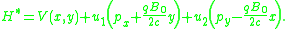
The next step is to apply the consistency conditions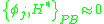 , which in this case become

These are not secondary constraints, but conditions that fix and
and  . Therefore, there are no secondary constraints and the arbitrary coefficients are completely determined, indicating that there are no unphysical degrees of freedom.
If one plugs in with the values of and
and  , then one can see that the equations for motion are


which are self-consistent and the same as the Lagrangian equations of motion.
A simple calculation confirms that and
and  are second class constraints since
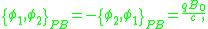
hence the matrix looks like
which is easily inverted to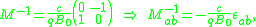
where is the Levi-Civita symbol
. Thus, the Dirac brackets are defined to be
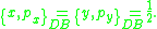
If one always uses the Dirac bracket instead of the Poisson bracket then there is no issue about the order of applying constraints and evaluating expressions, since the Dirac bracket of anything weakly zero is strongly equal to zero. This means that one can just use the naive Hamiltonian with Dirac brackets, and get the correct equations of motion, which one can easily confirm. To quantize the system, the Dirac brackets between all of the phase space variables are needed. The nonvanishing Dirac brackets for this system are below.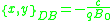
Therefore, the correct implementation of canonical quantization imposes the following commutation relations: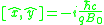
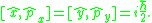
Interestingly, this example has a nonvanishing commutator between and
and  , which means this is a noncommutative geometry
. Since the two coordinates do not commute, there will be an uncertainty principle
for the and
and  position.
Poisson bracket
In mathematics and classical mechanics, the Poisson bracket is an important binary operation in Hamiltonian mechanics, playing a central role in Hamilton's equations of motion, which govern the time-evolution of a Hamiltonian dynamical system...
developed by Paul Dirac
Paul Dirac
Paul Adrien Maurice Dirac, OM, FRS was an English theoretical physicist who made fundamental contributions to the early development of both quantum mechanics and quantum electrodynamics...
to correctly treat systems with second class constraints
Second class constraints
In a constrained Hamiltonian system, a dynamical quantity is second class if its Poisson bracket with at least one constraint is nonvanishing...
in Hamiltonian mechanics
Hamiltonian mechanics
Hamiltonian mechanics is a reformulation of classical mechanics that was introduced in 1833 by Irish mathematician William Rowan Hamilton.It arose from Lagrangian mechanics, a previous reformulation of classical mechanics introduced by Joseph Louis Lagrange in 1788, but can be formulated without...
and canonical quantization
Canonical quantization
In physics, canonical quantization is a procedure for quantizing a classical theory while attempting to preserve the formal structure of the classical theory, to the extent possible. Historically, this was Werner Heisenberg's route to obtaining quantum mechanics...
. It is an important part of Dirac's development of Hamiltonian mechanics
Hamiltonian mechanics
Hamiltonian mechanics is a reformulation of classical mechanics that was introduced in 1833 by Irish mathematician William Rowan Hamilton.It arose from Lagrangian mechanics, a previous reformulation of classical mechanics introduced by Joseph Louis Lagrange in 1788, but can be formulated without...
to handle more general Lagrangian
Lagrangian
The Lagrangian, L, of a dynamical system is a function that summarizes the dynamics of the system. It is named after Joseph Louis Lagrange. The concept of a Lagrangian was originally introduced in a reformulation of classical mechanics by Irish mathematician William Rowan Hamilton known as...
s. More abstractly the two form implied from the Dirac bracket is the restriction of the symplectic form
Symplectic manifold
In mathematics, a symplectic manifold is a smooth manifold, M, equipped with a closed nondegenerate differential 2-form, ω, called the symplectic form. The study of symplectic manifolds is called symplectic geometry or symplectic topology...
to the constraint surface in phase space
Phase space
In mathematics and physics, a phase space, introduced by Willard Gibbs in 1901, is a space in which all possible states of a system are represented, with each possible state of the system corresponding to one unique point in the phase space...
.
This article assumes familiarity with the standard Lagrangian
Lagrangian
The Lagrangian, L, of a dynamical system is a function that summarizes the dynamics of the system. It is named after Joseph Louis Lagrange. The concept of a Lagrangian was originally introduced in a reformulation of classical mechanics by Irish mathematician William Rowan Hamilton known as...
and Hamiltonian
Hamiltonian mechanics
Hamiltonian mechanics is a reformulation of classical mechanics that was introduced in 1833 by Irish mathematician William Rowan Hamilton.It arose from Lagrangian mechanics, a previous reformulation of classical mechanics introduced by Joseph Louis Lagrange in 1788, but can be formulated without...
formalisms, and their connection to canonical quantization
Canonical quantization
In physics, canonical quantization is a procedure for quantizing a classical theory while attempting to preserve the formal structure of the classical theory, to the extent possible. Historically, this was Werner Heisenberg's route to obtaining quantum mechanics...
. The details of Dirac's modified Hamiltonian formalism are summarized to put the Dirac bracket in context.
Inadequacy of the standard Hamiltonian procedure
The standard development of Hamiltonian mechanics is inadequate in several specific situations:- When the Lagrangian is at most linear in the velocity of at least one coordinate; in which case, the definition of the canonical momentum leads to a constraint. This is the most frequent reason to resort to Dirac brackets. For instance, the Lagrangian (density) for any fermionFermionIn particle physics, a fermion is any particle which obeys the Fermi–Dirac statistics . Fermions contrast with bosons which obey Bose–Einstein statistics....
is of this form. - When there are gaugeGauge fixingIn the physics of gauge theories, gauge fixing denotes a mathematical procedure for coping with redundant degrees of freedom in field variables. By definition, a gauge theory represents each physically distinct configuration of the system as an equivalence class of detailed local field...
(or other unphysical) degrees of freedom which need to be fixed. - When there are any other constraints that one wishes to impose in phase space.
Example of a Lagrangian linear in velocity
An example in classical mechanicsClassical mechanics
In physics, classical mechanics is one of the two major sub-fields of mechanics, which is concerned with the set of physical laws describing the motion of bodies under the action of a system of forces...
is a particle with charge
and mass fixed in the - plane with a strong constant, homogeneous magnetic field pointing in the -direction with strength . The Lagrangian for the system with an appropriate choice of parameters iswhere
is the vector potentialVector potential
In vector calculus, a vector potential is a vector field whose curl is a given vector field. This is analogous to a scalar potential, which is a scalar field whose negative gradient is a given vector field....
for the magnetic field,
; is the speed of light in vacuum; and is an arbitrary external scalar potential. We useas our vector potential. Here, the hats indicate unit vectors. Later in the article they are used to distinguish quantum mechanical operators from their classical analogs. The usage should be clear from the context.
Explicitly, the Lagrangian
Lagrangian
The Lagrangian, L, of a dynamical system is a function that summarizes the dynamics of the system. It is named after Joseph Louis Lagrange. The concept of a Lagrangian was originally introduced in a reformulation of classical mechanics by Irish mathematician William Rowan Hamilton known as...
becomes
which leads to the equations of motion
Now consider the limit where
which corresponds to a very large magnetic field. In which case, one can drop the mass term to find an approximate Lagrangianand first order equations of motion
Notice that this approximate Lagrangian is linear in the velocities which is one of the conditions under which the standard Hamiltonian procedure breaks down. While this example has been motivated as an approximation, the Lagrangian under consideration is perfectly allowable and leads to consistent equations of motion in the Lagrangian formalism.
Following the Hamiltonian procedure, the canonical momenta associated with the coordinates are
which are unusual in that they are not invertible to the velocities. A Legendre transformation
Legendre transformation
In mathematics, the Legendre transformation or Legendre transform, named after Adrien-Marie Legendre, is an operation that transforms one real-valued function of a real variable into another...
produces the Hamiltonian,
Note that this "naive" Hamiltonian has no dependence on the momenta, which means that equations of motion from Hamilton's equations are inconsistent; the Hamiltonian procedure has broken down. One might try to fix the problem by sometimes expressing the coordinates as momenta and sometimes as coordinates; however, this is neither a general nor rigorous solution. This last comment gets at the heart of the matter, that the definition of the canonical momenta implies a constraint on phase space (between momenta and coordinates) that was never taken into account.
Generalized Hamiltonian procedure
In Lagrangian mechanics, if the system has holonomic constraintsHolonomic constraints
In a system of point particles, holonomic constraints are relations between the coordinates and time which can be expressed in the following form:...
, then one generally adds Lagrange multipliers
Lagrange multipliers
In mathematical optimization, the method of Lagrange multipliers provides a strategy for finding the maxima and minima of a function subject to constraints.For instance , consider the optimization problem...
to the Lagrangian to account for them. The extra terms vanish when the constraints are satisfied, thereby forcing the path of stationary action to be on the constraint surface. In this case, going to the Hamiltonian formalism introduces a constraint on phase space in Hamiltonian mechanics, but the solution is similar.
Before proceeding, it is useful to understand the notions of weak equality and strong equality. Two functions on phase space,
and , are weakly equal if they are equal when the equations of motion are satisfied or on shellOn shell and off shell
In physics, particularly in quantum field theory, configurations of a physical system that satisfy classical equations of motion are called on shell, and those that do not are called off shell....
, denoted
. If and are equal on and off shell, then they are called strongly equal, written . It is important to note that in order to get the right answer no weak equations may be used before evaluating derivatives or Poisson brackets.The new procedure works as follows, start with a Lagrangian and define the canonical momenta in the usual way. Some of those definitions may not be invertible and instead give a constraint in phase space (as above). Constraints derived in this way or imposed from the beginning of the problem are called primary constraints. The constraints, labeled
, must weakly vanish, .Next, one finds the naive Hamiltonian,
, in the usual way via a Legendre transformation, exactly as in the above example. Note that the Hamiltonian can always be written as a function of 's and 's only, even if the velocities cannot be inverted into functions of the momenta.Generalizing the Hamiltonian
Dirac argues that we should generalize the Hamiltonian (somewhat analogously to the method of Lagrange multipliers) towhere the
are not constants but functions of the coordinates and momenta. Since this new Hamiltonian is the most general function of coordinates and momenta weakly equal to the naive Hamiltonian, is the broadest generalization of the Hamiltonian possible.To illuminate the
more, consider how one gets the equations of motion from the naive Hamiltonian in the standard procedure. One expands the variation of the Hamiltonian out in two ways and sets them equal (using a somewhat abbreviated notation with suppressed indices and sums):where the second equality holds after simplifying with the Euler-Lagrange equations of motion and the definition of canonical momentum. From this equality, one deduces the equations of motion in the Hamiltonian formalism from
where the weak equality symbol is no longer displayed explicitly, since by definition the equations of motion only hold weakly. In the present context, one cannot simply set the coefficients of
and separately to zero, since the variations are somewhat restricted by the constraints. In particular, the variations must be tangent to the constraint surface.One can demonstrate the solution to
for the variations
and restricted by the constraints (assuming the constraints satisfy some regularity conditions) is generallywhere the
are arbitrary functions.Using this result, the equations of motion become
where the
are functions of coordinates and velocities that can be determined, in principle, from the second equation of motion above. The Legendre transform between the Lagrangian formalism and the Hamiltonian formalism is saved at the cost of adding new variables.Consistency conditions
The equations of motion become more compact when using the Poisson bracket, since if is some function of the coordinates and momenta thenif one assumes that the Poisson bracket with the
(functions of the velocity) exist; this causes no problems since the contribution weakly vanishes. Now, there are some consistency conditions which must be satisfied in order for this formalism to make sense. If the constraints are going to be satisfied, then their equations of motion must weakly vanish, that is, we requireThere are four different types of conditions that can result from the above:
- An equation that is inherently false, such as
 .
. - An equation that is identically true, possibly after using one of our primary constraints.
- An equation that places new constraints on our coordinates and momenta, but is independent of the
 .
. - An equation that helps fix the
 .
.
The first case indicates that the starting Lagrangian gives inconsistent equations of motion, such as
. The second case does not contribute anything new.The third case gives new constraints in phase space. A constraint derived in this manner is called a secondary constraint. Upon finding the secondary constraint one should add it to the extended Hamiltonian and check the new consistency conditions, which may result in still more constraints. Iterate this process until there are no more constraints. The distinction between primary and secondary constraints is largely an artificial one (i.e. a constraint for the same system can be primary or secondary depending on the Lagrangian), so this article does not distinguish between them from here on. Assuming the consistency condition has been iterated until all of the constraints have been found, then
will index all of them. Note this article uses secondary constraint to mean any constraint that was not initially in the problem or derived from the definition of canonical momenta; some authors distinguish between secondary constraints, tertiary constraints, et cetera.Finally, the last case helps fix the
. If, at the end of this process, the are not completely determined then that means there are unphysical (gauge) degrees of freedom in the system. Once all of the constraints (primary and secondary) are added to the naive Hamiltonian and the solutions to the consistency conditions for the are plugged in the result is called the total Hamiltonian. Fixing the 
The must solve a set of inhomogeneous linear equations of the formThe above equation must possess at least one solution, since otherwise the initial Lagrangian is inconsistent; however, in systems with gauge degrees of freedom, the solution will not be unique. The most general solution is of the form
where
is a particular solution and is the most general solution to the homogeneous equationThe most general solution will be a linear combination of linearly independent solutions to the above homogeneous equation. The number of linearly independent solutions equals the number of
(which is the same as the number of constraints) minus the number of consistency conditions of the fourth type (in previous subsection). This is the number of unphysical degrees of freedom in the system. Labeling the linear independent solutions where the index runs from 1 to the number of unphysical degrees of freedom, the general solution to the consistency conditions is of the formwhere the
are completely arbitrary functions of time. A different choice of the corresponds to a gauge transformation and should leave the physical state of the system unchanged.The total Hamiltonian
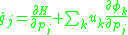
At this point, it is natural to introduce the total Hamiltonianand what is denoted
The time evolution of a function on the phase space,
is governed byLater, the extended Hamiltonian is introduced. For gauge-invariant (physically measurable quantities) quantities all of the Hamiltonians should give the same time evolution since they are all weakly equivalent. It is only for nongauge-invariant quantities that the distinction becomes important.
The Dirac bracket
Above is everything needed to find the equations of motion in Dirac's modified Hamiltonian procedure. Having the equations of motion, however, is not the endpoint for theoretical considerations. If one wants to canonically quantize a general system, then one needs the Dirac brackets.Before defining Dirac brackets, first class and second class constraints need to be introduced. We call a function
of coordinates and momenta first class if its Poisson bracket with all of the constraints weakly vanishes, that is,for all
. Note that the only quantities that weakly vanish are the constraints , and therefore anything that weakly vanishes must be strongly equal to a linear combination of the constraints. One can demonstrate that the Poisson bracket of two first class quantities must also be first class. The first class constraints are intimately connected with the unphysical degrees of freedom mentioned earlier. Namely, the number of independent first class constraints is equal to the number of unphysical degrees of freedom, and furthermore the primary first class constraints generate gauge transformations. Dirac further postulated that all secondary first class constraints are generators of gauge transformations, which turns out to be false; however, typically one operates under the assumption that all first class constraints generate gauge transformations when using this treatment.When the first class secondary constraints are added into the Hamiltonian with arbitrary
as the first class primary constraints are added to arrive at the total Hamiltonian, then one obtains the extended Hamiltonian. The extended Hamiltonian gives the most general possible time evolution for any gauge-dependent quantities, and may actually generalize the equations of motion from those of the Lagrangian formalism.For the purposes of introducing the Dirac bracket, of more immediate interest are the second class constraints. Second class constraints are constraints that have nonvanishing Poisson bracket with at least one other constraint. For instance, consider constraints
and whose Poisson bracket is simply a constant, ,Now, suppose one wishes to employ canonical quantization, then the phase space coordinates become operators whose commutators become
times their classical Poisson bracket. Assuming there are no ordering issues that give rise to new quantum corrections, this implies thatwhere the hats emphasize the fact that the constraints are operators. On the one hand, canonical quantization gives the above commutation relation, but on the other hand
and are constraints that must vanish on physical states, whereas the right hand side cannot vanish. This example illustrates the need for a generalization of the Poisson bracket that respects the system's constraints, and leads to a consistent quantization procedure.The new bracket should be bilinear, antisymmetric, satisfy the Jacobi identity as does the Poisson bracket, reduce to the Poisson bracket for unconstrained systems, and additionally the bracket of any constraint with any other quantity must vanish. At this point, the second class constraints will be labeled
. Define a matrix with entriesIn which case, the Dirac bracket of two functions on phase space,
and , is defined aswhere
denotes the entry of 's inverse matrix. Dirac proved that will always be invertible. It is straightforward to check that the above definition of the Dirac bracket satisfies all of the desired properties. When using canonical quantization with a constrained Hamiltonian system, the commutator of the operators is set to times their classical Dirac bracket. Since the Dirac bracket respects the constraints, one does not have to be careful about evaluating all brackets before using any weak equations as is true with the Poisson bracket.Note that while the Poisson bracket of a bosonic (Grassmann even) variables with itself must vanish, the Poisson bracket of a fermion represented as a Grassmann variables
Grassmann number
In mathematical physics, a Grassmann number, named after Hermann Grassmann, is a mathematical construction which allows a path integral representation for Fermionic fields...
with itself need not vanish. This means that in the fermionic case it is possible for there to be an odd number of second class constraints.
Finishing the example
Returning to the above example, the naive Hamiltonian and the two primary constraints areTherefore the extended Hamiltonian can be written
The next step is to apply the consistency conditions
, which in this case becomeThese are not secondary constraints, but conditions that fix
and . Therefore, there are no secondary constraints and the arbitrary coefficients are completely determined, indicating that there are no unphysical degrees of freedom.If one plugs in with the values of
and , then one can see that the equations for motion arewhich are self-consistent and the same as the Lagrangian equations of motion.
A simple calculation confirms that
and are second class constraints sincehence the matrix looks like
which is easily inverted to
where
is the Levi-Civita symbolLevi-Civita symbol
The Levi-Civita symbol, also called the permutation symbol, antisymmetric symbol, or alternating symbol, is a mathematical symbol used in particular in tensor calculus...
. Thus, the Dirac brackets are defined to be
If one always uses the Dirac bracket instead of the Poisson bracket then there is no issue about the order of applying constraints and evaluating expressions, since the Dirac bracket of anything weakly zero is strongly equal to zero. This means that one can just use the naive Hamiltonian with Dirac brackets, and get the correct equations of motion, which one can easily confirm. To quantize the system, the Dirac brackets between all of the phase space variables are needed. The nonvanishing Dirac brackets for this system are below.
Therefore, the correct implementation of canonical quantization imposes the following commutation relations:
Interestingly, this example has a nonvanishing commutator between
and , which means this is a noncommutative geometryNoncommutative geometry
Noncommutative geometry is a branch of mathematics concerned with geometric approach to noncommutative algebras, and with construction of spaces which are locally presented by noncommutative algebras of functions...
. Since the two coordinates do not commute, there will be an uncertainty principle
Uncertainty principle
In quantum mechanics, the Heisenberg uncertainty principle states a fundamental limit on the accuracy with which certain pairs of physical properties of a particle, such as position and momentum, can be simultaneously known...
for the
and position.See also
- First class constraintFirst class constraintIn a constrained Hamiltonian system, a dynamical quantity is called a first class constraint if its Poisson bracket with all the other constraints vanishes on the constraint surface .-Poisson brackets:In Hamiltonian mechanics, consider a symplectic manifold M with a smooth Hamiltonian over...
- Second class constraintsSecond class constraintsIn a constrained Hamiltonian system, a dynamical quantity is second class if its Poisson bracket with at least one constraint is nonvanishing...
- Hamiltonian mechanicsHamiltonian mechanicsHamiltonian mechanics is a reformulation of classical mechanics that was introduced in 1833 by Irish mathematician William Rowan Hamilton.It arose from Lagrangian mechanics, a previous reformulation of classical mechanics introduced by Joseph Louis Lagrange in 1788, but can be formulated without...
- Poisson bracketPoisson bracketIn mathematics and classical mechanics, the Poisson bracket is an important binary operation in Hamiltonian mechanics, playing a central role in Hamilton's equations of motion, which govern the time-evolution of a Hamiltonian dynamical system...
- Canonical quantizationCanonical quantizationIn physics, canonical quantization is a procedure for quantizing a classical theory while attempting to preserve the formal structure of the classical theory, to the extent possible. Historically, this was Werner Heisenberg's route to obtaining quantum mechanics...
- LagrangianLagrangianThe Lagrangian, L, of a dynamical system is a function that summarizes the dynamics of the system. It is named after Joseph Louis Lagrange. The concept of a Lagrangian was originally introduced in a reformulation of classical mechanics by Irish mathematician William Rowan Hamilton known as...
- Faddeev–Jackiw bracket
- Quantum deformation of the Dirac bracket