

Wilkinson's polynomial
Encyclopedia
Numerical analysis
Numerical analysis is the study of algorithms that use numerical approximation for the problems of mathematical analysis ....
, Wilkinson's polynomial is a specific polynomial
Polynomial
In mathematics, a polynomial is an expression of finite length constructed from variables and constants, using only the operations of addition, subtraction, multiplication, and non-negative integer exponents...
which was used by James H. Wilkinson
James H. Wilkinson
James Hardy Wilkinson was a prominent figure in the field of numerical analysis, a field at the boundary of applied mathematics and computer science particularly useful to physics and engineering.-Early life:...
in 1963 to illustrate a difficulty when finding the root
Root-finding algorithm
A root-finding algorithm is a numerical method, or algorithm, for finding a value x such that f = 0, for a given function f. Such an x is called a root of the function f....
of a polynomial: the location of the roots can be very sensitive to perturbations in the coefficients of the polynomial.
The polynomial is

Sometimes, the term Wilkinson's polynomial is also used to refer to some other polynomials appearing in Wilkinson's discussion.
Background
Wilkinson's polynomial arose in the study of algorithms for finding the roots of a polynomial
It is a natural question in numerical analysis to ask whether the problem of finding the roots of p from the coefficients ci is well-conditioned
Condition number
In the field of numerical analysis, the condition number of a function with respect to an argument measures the asymptotically worst case of how much the function can change in proportion to small changes in the argument...
. That is, we hope that a small change in the coefficients will lead to a small change in the roots. Unfortunately, that is not the case here.
The problem is ill-conditioned when the polynomial has a multiple root. For instance, the polynomial x2 has a double root at x = 0. However, the polynomial x2−ε (a perturbation of size ε) has roots at ±√ε, which is much bigger than ε when ε is small.
It is therefore natural to expect that ill-conditioning also occurs when the polynomial has zeros which are very close. However, the problem may also be extremely ill-conditioned for polynomials with well-separated zeros. Wilkinson used the polynomial w(x) to illustrate this point (Wilkinson 1963).
In 1984, he described the personal impact of this discovery:
- Speaking for myself I regard it as the most traumatic experience in my career as a numerical analyst.
Wilkinson's polynomial is often used to illustrate the undesirability of naively computing eigenvalues of a matrix by first calculating the coefficients of the matrix's characteristic polynomial
Characteristic polynomial
In linear algebra, one associates a polynomial to every square matrix: its characteristic polynomial. This polynomial encodes several important properties of the matrix, most notably its eigenvalues, its determinant and its trace....
and then finding its roots, since using the coefficients as an intermediate step may introduce an extreme ill-conditioning even if the original problem was well conditioned.
Conditioning of Wilkinson's polynomial
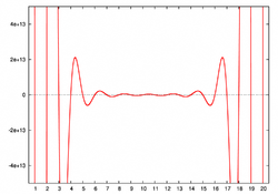
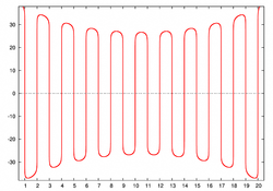
Wilkinson's polynomial
clearly has 20 roots, located at x = 1, 2, …, 20. These roots are far apart. However, the polynomial is still very ill-conditioned.
Expanding the polynomial, one finds
 |
 |
 |
|
 |
|
 |
|
 |
|
 |
|
 |
|
 |
|
 |
If the coefficient of x19 is decreased from −210 by 2−23 to −210.0000001192, then the polynomial value w(20) decreases from 0 to −2−232019 = −6.25×10¹⁷, and the root at x = 20 grows to x ≈ 20.8 . The roots at x = 18 and x = 19 collide into a double root at x ≈ 18.62 which turns into a pair of complex conjugate roots at x ≈ 19.5±1.9i as the perturbation increases further. The 20 roots become (to 5 decimals)
| 1.00000 | 2.00000 | 3.00000 | 4.00000 | 5.00000 |
| 6.00001 | 6.99970 | 8.00727 | 8.91725 | 20.84691 |
| 10.09527± 0.64350i |
11.79363± 1.65233i |
13.99236± 2.51883i |
16.73074± 2.81262i |
19.50244± 1.94033i |
Some of the roots are greatly displaced, even though the change to the coefficient is tiny and the original roots seem widely spaced. Wilkinson showed by the stability analysis discussed in the next section that this behavior is related to the fact that some roots α (such as α = 15) have many roots β that are "close" in the sense that |α−β| is smaller than |α|.
Wilkinson chose the perturbation of 2−23 because his Pilot ACE
Pilot ACE
The Pilot ACE was one of the first computers built in the United Kingdom, at the National Physical Laboratory in the early 1950s.It was a preliminary version of the full ACE, which had been designed by Alan Turing. After Turing left NPL , James H...
computer had 30-bit floating point
Floating point
In computing, floating point describes a method of representing real numbers in a way that can support a wide range of values. Numbers are, in general, represented approximately to a fixed number of significant digits and scaled using an exponent. The base for the scaling is normally 2, 10 or 16...
significand
Significand
The significand is part of a floating-point number, consisting of its significant digits. Depending on the interpretation of the exponent, the significand may represent an integer or a fraction.-Examples:...
s, so for numbers around 210, 2−23 was an error in the first bit position not represented in the computer. The two real numbers, −210 and −210 − 2−23, are represented by the same floating point number, which means that 2−23 is the unavoidable error in representing a real coefficient close to −210 by a floating point number on that computer. The perturbation analysis shows that 30-bit coefficient precision
Precision (arithmetic)
The precision of a value describes the number of digits that are used to express that value. In a scientific setting this would be the total number of digits or, less commonly, the number of fractional digits or decimal places...
is insufficient for separating the roots of Wilkinson's polynomial.
Stability analysis
Suppose that we perturb a polynomial p(x) = Π (x−αj)with roots αj by adding a small multiple t·c(x) of a polynomial c(x), and ask how this affects the roots αj. To first order, the change in the roots will be controlled by the derivative

When the derivative is large, the roots will be less stable under variations of t, and conversely if this derivative is small the roots will be stable. In particular,
if αj is a multiple root, then the denominator vanishes. In this case, αj is usually not differentiable with respect to t (unless c happens to vanish there), and the roots will be extremely unstable.
For small values of t the perturbed root is given by the power series expansion in t

and one expects problems when |t| is larger than the radius of convergence of this power series, which is given by the smallest value of |t| such that the root αj becomes multiple. A very crude estimate for this radius takes half the distance from αj to the nearest root, and divides by the derivative above.
In the example of Wilkinson's polynomial of degree 20, the roots are given by αj = j for j = 1, …, 20, and c(x) is equal to x19.
So the derivative is given by

This shows that the root αj will be less stable if there are many roots
αk close to αj, in the sense that the distance
|αj−αk| between them is smaller than |αj|.
Example. For the root α1 = 1, the derivative is equal to
1/19! which is very small; this root is stable even for large changes in t. This is because all the other roots β are a long way from it, in the sense that |α1−β| = 1, 2, 3, ..., 19 is larger than |α1| = 1.
For example even if t is as large as –10000000000, the root α1 only changes from 1 to about 0.99999991779380 (which is very close to the first order approximation 1+t/19! ≈ 0.99999991779365). Similarly, the other small roots of Wilkinson's polynomial are insensitive to changes in t.
Example. On the other hand, for the root α20 = 20, the derivative is equal to
−2019/19! which is huge (about 43000000), so this root is very sensitive to small changes in t. The other roots β are close to α20, in the sense that |β − α20| = 1, 2, 3, ..., 19 is less than |α20| = 20. For t = −2−23 the first-order approximation 20 − t·2019/19! = 25.137... to the perturbed root 20.84... is terrible; this is even more obvious for the root α19 where the perturbed root has a large imaginary part but the first-order approximation (and for that matter all higher-order approximations) are real. The reason for this discrepancy is that |t| ≈ 0.000000119 is greater than the radius of convergence of the power series mentioned above (which is about 0.0000000029, somewhat smaller than the value 0.00000001 given by the crude estimate) so the linearized theory does not apply. For a value such as t = 0.000000001 that is significantly smaller than this radius of convergence, the first-order approximation 19.9569... is reasonably close to the root 19.9509...
At first sight the roots α1 = 1 and α20 = 20 of Wilkinson's polynomial appear to be similar, as they are on opposite ends of a symmetric line of roots, and have the same set of distances 1, 2, 3, ..., 19 from other roots. However the analysis above shows that this is grossly misleading: the root α20 = 20 is less stable than α1 = 1 (to small perturbations in the coefficient of x19) by a factor of 2019 = 5242880000000000000000000.
Wilkinson's second example
The second example considered by Wilkinson is
The twenty zeros of this polynomial are in a geometric progression with common ratio 2, and hence the quotient

cannot be large. Indeed, the zeros of w2 are quite stable to large relative changes in the coefficients.
The effect of the basis
The expansion
expresses the polynomial in a particular basis, namely that of the monomials. If the polynomial is expressed in another basis, then the problem of finding its roots may cease to be ill-conditioned. For example, in a Lagrange form
Lagrange polynomial
In numerical analysis, Lagrange polynomials are used for polynomial interpolation. For a given set of distinct points x_j and numbers y_j, the Lagrange polynomial is the polynomial of the least degree that at each point x_j assumes the corresponding value y_j...
, a small change in one (or several) coefficients need not change the roots too much. Indeed, the basis polynomials for interpolation at the points 0, 1, 2, …, 20 are

Every polynomial (of degree 20 or less) can be expressed in this basis:

For Wilkinson's polynomial, we find

Given the definition of the Lagrange basis polynomial ℓ0(x), a change in the coefficient d0 will produce no change in the roots of w. However, a perturbation in the other coefficients (all equal to zero) will slightly change the roots. Therefore, Wilkinson's polynomial is well-conditioned in this basis.