
.gif)
Triangulation (computer vision)
Encyclopedia
In computer vision
triangulation refers to the process of determining a point in 3D space given its projections onto two, or more, images. In order to solve this problem it is necessary to know the parameters of the camera projection function from 3D to 2D for the cameras involved, in the simplest case represented by the camera matrices
. Triangulation is sometimes also referred to as reconstruction.
The triangulation problem is in theory trivial, each point in an image corresponds to a line in 3D space such that all points on the line are projected to that first point in the image. If a pair of corresponding points
in two, or more images, can be found it must be the case that they are the projection of a common 3D point x. The set of lines generated by the image points must intersect at x and the algebraic formulation of the coordinates of x can be computed in a variety of ways, as is presented below.
In practice, however, the coordinates of image points cannot be measured with arbitrary accuracy. Instead, various types of noise, such as geometric noise from lens distortion or interest point detection error, lead to inaccuracies in the measured image coordinates. As a consequence, the lines generated by the corresponding image points do not always intersect in 3D space. The problem, then, is to find a 3D point which optimally fits the measured image points. In the literature there are multiple proposals for how to define optimality and how to find the optimal 3D point. Since they are based on different optimality criteria, the various methods produce different estimates of the 3D point x when noise is involved.
. Generalization from these assumptions are discussed here.
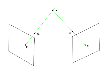
 The image to the left illustrates the epipolar geometry
of a pair of stereo cameras of pinhole model
. A point x in 3D space is projected onto the respective image plane along a line (green) which goes through the camera's focal point
, and
and  , resulting in the two corresponding image points
  and
and  . If
. If  and
and  is given and the geometry of the two cameras are known, the two projection lines can be determined and it must be the case that they intersect at point x. Using basic linear algebra
that intersection point can be determined in a straightforward way.
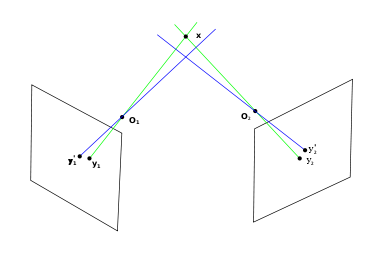
The image to the right shows the real case. The position of the image points and
and  cannot be measured exactly. The reason is a combination of factors such as
As a consequence, the measured image points are and
and  instead of
  and
and  . However, their projection lines (blue) do not have to intersect in 3D space or come close to x. In fact, these lines intersect if and only if
  and
and  satisfy the epipolar constraint defined by the fundamental matrix. Given the measurement noise in
  and
and  it is rather likely that the epipolar constraint is not satisfied and the projection lines do not intersect.
This observation leads to the problem which is solved in triangulation. Which 3D point xest is the best estimate of x given and
and  and the geometry of the cameras? The answer is often found by defining an error measure which depends on xest and then minimize this error. In the following some of the various methods for computing xest presented in the literature are briefly described.
All triangulation methods produce xest = x in the case that and
and  , that is, when the epipolar constraint is satisfied (except for singular points, see below). It is what happens when the constraint is not satisfied which differs between the methods.
 such that
where are the homogeneous coordinates of the detected image points and
  are the camera matrices. x is the homogeneous representation of the resulting 3D point. The
  sign implies that
  is only required to produce a vector which is equal to x up to a multiplication by a non-zero scalar since homogeneous vectors are involved.
Before looking at the specific methods, that is, specific functions , there are some general concepts related to the methods that need to be explained. Which triangulation method is chosen for a particular problem depends to some extent on these characteristics.
 . A point in this subset is then a singularity of the triangulation method. The reason for the failure can be that some equation system to be solved is under-determined or that the projective representation of xest becomes the zero vector for the singular points.
For a homogeneous representation of 3D coordinates, the most general transformation is a projective transformation, represented by a matrix
  . If the homogeneous coordinates are transformed according to

then the camera matrices must transform as

to produce the same homogeneous image coordinates
If the triangulation function is invariant to
  then the following relation must be valid

from which follows that
 for all
For each triangulation method, it can be determined if this last relation is valid. If it is, it may be satisfied only for a subset of the projective transformations, for example, rigid or affine transformations.
 is only an abstract representation of a computation which, in practice, may be relatively complex. Some methods result in a
  which is a closed-form continuous function while others need to be decomposed into a series of computational steps involving, for example, SVD
or finding the roots of a polynomial. Yet another class of methods results in which must rely on iterative estimation of some parameters. This means that both the computation time and the complexity of the operations involved may vary between the different methods.
 and
and  has a corresponding projection line (blue in the right image above), here denoted as
  and
and  , which can be determined given the camera matrices
  . Let
. Let  be a distance function between a 3D line and a 3D point such that
 the Euclidean distance between
  and
and  .
.
The mid-point method finds the point xest which minimizes
It turns out that xest lies exactly at the middle of the shortest line segment which joins the two projection lines.
Computer vision
Computer vision is a field that includes methods for acquiring, processing, analysing, and understanding images and, in general, high-dimensional data from the real world in order to produce numerical or symbolic information, e.g., in the forms of decisions...
triangulation refers to the process of determining a point in 3D space given its projections onto two, or more, images. In order to solve this problem it is necessary to know the parameters of the camera projection function from 3D to 2D for the cameras involved, in the simplest case represented by the camera matrices
Camera matrix
In computer vision a camera matrix or projection matrix is a 3 \times 4 matrix which describes the mapping of a pinhole camera from 3D points in the world to 2D points in an image....
. Triangulation is sometimes also referred to as reconstruction.
The triangulation problem is in theory trivial, each point in an image corresponds to a line in 3D space such that all points on the line are projected to that first point in the image. If a pair of corresponding points
Correspondence problem
The correspondence problem tries to figure out which parts of an image correspond to which parts of another image, after the camera has moved, time has elapsed, and/or the objects have moved around.-Overview:...
in two, or more images, can be found it must be the case that they are the projection of a common 3D point x. The set of lines generated by the image points must intersect at x and the algebraic formulation of the coordinates of x can be computed in a variety of ways, as is presented below.
In practice, however, the coordinates of image points cannot be measured with arbitrary accuracy. Instead, various types of noise, such as geometric noise from lens distortion or interest point detection error, lead to inaccuracies in the measured image coordinates. As a consequence, the lines generated by the corresponding image points do not always intersect in 3D space. The problem, then, is to find a 3D point which optimally fits the measured image points. In the literature there are multiple proposals for how to define optimality and how to find the optimal 3D point. Since they are based on different optimality criteria, the various methods produce different estimates of the 3D point x when noise is involved.
Introduction
In the following, it is assumed that triangulation is made on corresponding image points from two views generated by pinhole camerasPinhole camera model
The pinhole camera model describes the mathematical relationship between the coordinates of a 3D point and its projection onto the image plane of an ideal pinhole camera, where the camera aperture is described as a point and no lenses are used to focus light...
. Generalization from these assumptions are discussed here.
Epipolar geometry
Epipolar geometry is the geometry of stereo vision. When two cameras view a 3D scene from two distinct positions, there are a number of geometric relations between the 3D points and their projections onto the 2D images that lead to constraints between the image points...
of a pair of stereo cameras of pinhole model
Pinhole camera model
The pinhole camera model describes the mathematical relationship between the coordinates of a 3D point and its projection onto the image plane of an ideal pinhole camera, where the camera aperture is described as a point and no lenses are used to focus light...
. A point x in 3D space is projected onto the respective image plane along a line (green) which goes through the camera's focal point
Focus (optics)
In geometrical optics, a focus, also called an image point, is the point where light rays originating from a point on the object converge. Although the focus is conceptually a point, physically the focus has a spatial extent, called the blur circle. This non-ideal focusing may be caused by...
,
and , resulting in the two corresponding image points and . If and is given and the geometry of the two cameras are known, the two projection lines can be determined and it must be the case that they intersect at point x. Using basic linear algebraLinear algebra
Linear algebra is a branch of mathematics that studies vector spaces, also called linear spaces, along with linear functions that input one vector and output another. Such functions are called linear maps and can be represented by matrices if a basis is given. Thus matrix theory is often...
that intersection point can be determined in a straightforward way.
The image to the right shows the real case. The position of the image points
and cannot be measured exactly. The reason is a combination of factors such as- Geometric distortion, for example lens distortion, which means that the 3D to 2D mapping of the camera deviates from the pinhole camera modelPinhole camera modelThe pinhole camera model describes the mathematical relationship between the coordinates of a 3D point and its projection onto the image plane of an ideal pinhole camera, where the camera aperture is described as a point and no lenses are used to focus light...
. To some extent these errors can be compensated for, leaving a residual geometric error. - A single ray of light from x is dispersed in the lens system of the cameras according to a point spread functionPoint spread functionThe point spread function describes the response of an imaging system to a point source or point object. A more general term for the PSF is a system's impulse response, the PSF being the impulse response of a focused optical system. The PSF in many contexts can be thought of as the extended blob...
. The recovery of the corresponding image point from measurements of the dispersed intensity function in the images gives errors. - In digital camera the image intensity function is only measured in discrete sensor elements. Inexact interpolation of the discrete intensity function have to be used to recover the true one.
- The image points used for triangulation are often found using various types of feature extractors, for example of corners or interest points in general. There is an inherent localization error for any type of feature extraction based on neighborhood operations.
As a consequence, the measured image points are
and instead of and . However, their projection lines (blue) do not have to intersect in 3D space or come close to x. In fact, these lines intersect if and only if and satisfy the epipolar constraint defined by the fundamental matrix. Given the measurement noise in and it is rather likely that the epipolar constraint is not satisfied and the projection lines do not intersect.This observation leads to the problem which is solved in triangulation. Which 3D point xest is the best estimate of x given
and and the geometry of the cameras? The answer is often found by defining an error measure which depends on xest and then minimize this error. In the following some of the various methods for computing xest presented in the literature are briefly described.All triangulation methods produce xest = x in the case that
and , that is, when the epipolar constraint is satisfied (except for singular points, see below). It is what happens when the constraint is not satisfied which differs between the methods.Properties of triangulation methods
A triangulation method can be described in terms of a function such thatwhere
are the homogeneous coordinates of the detected image points and are the camera matrices. x is the homogeneous representation of the resulting 3D point. The sign implies that is only required to produce a vector which is equal to x up to a multiplication by a non-zero scalar since homogeneous vectors are involved.Before looking at the specific methods, that is, specific functions
, there are some general concepts related to the methods that need to be explained. Which triangulation method is chosen for a particular problem depends to some extent on these characteristics.Singularities
Some of the methods fail to correctly compute an estimate of x if it lies in a certain subset of the 3D space, correspondig to some combination of. A point in this subset is then a singularity of the triangulation method. The reason for the failure can be that some equation system to be solved is under-determined or that the projective representation of xest becomes the zero vector for the singular points.Invariance
In some applications, it is desirable that the triangulation is independent of the coordinate system used to represent 3D points; if the triangulation problem is formulated in one coordinate system and then transformed into another the resulting estimate xest should transform in the same way. This property is commonly referred to as invariance. Not every triangulation method assures invariance, at least not for general types of coordinate transformations.For a homogeneous representation of 3D coordinates, the most general transformation is a projective transformation, represented by a
matrix . If the homogeneous coordinates are transformed according tothen the camera matrices must transform as
to produce the same homogeneous image coordinates
If the triangulation function
is invariant to then the following relation must be validfrom which follows that
for all For each triangulation method, it can be determined if this last relation is valid. If it is, it may be satisfied only for a subset of the projective transformations, for example, rigid or affine transformations.
Computational complexity
The function is only an abstract representation of a computation which, in practice, may be relatively complex. Some methods result in a which is a closed-form continuous function while others need to be decomposed into a series of computational steps involving, for example, SVDSingular value decomposition
In linear algebra, the singular value decomposition is a factorization of a real or complex matrix, with many useful applications in signal processing and statistics....
or finding the roots of a polynomial. Yet another class of methods results in
which must rely on iterative estimation of some parameters. This means that both the computation time and the complexity of the operations involved may vary between the different methods.Mid-point method
Each of the two image points and has a corresponding projection line (blue in the right image above), here denoted as and , which can be determined given the camera matrices . Let be a distance function between a 3D line and a 3D point such that the Euclidean distance between and .The mid-point method finds the point xest which minimizes
It turns out that xest lies exactly at the middle of the shortest line segment which joins the two projection lines.