
Fractional cascading
Encyclopedia
In computer science
, fractional cascading is a technique to speed up a sequence of binary searches for the same value in a sequence of related data structures. The first binary search in the sequence takes a logarithmic amount of time, as is standard for binary searches, but successive searches in the sequence are faster. The original version of fractional cascading, introduced in two papers by Chazelle
and Guibas
in 1986, combined the idea of cascading, originating in range searching
data structures of and , with the idea of fractional sampling, which originated in . Later authors introduced more complex forms of fractional cascading that allow the data structure to be maintained as the data changes by a sequence of discrete insertion and deletion events.
s, such that the total length Σ|Li| of all lists is n, and must process them so that we can perform binary searches for a query value q in each of the k lists. For instance, with k = 4 and n = 17,
The simplest solution to this searching problem is just to store each list separately. If we do so, the space requirement is O(n), but the time to perform a query is O(k log(n/k)), as we must perform a separate binary search in each of k lists. The worst case for querying this structure occurs when each of the k lists has equal size n/k, so each of the k binary searches involved in a query takes time O(log(n/k)).
A second solution allows faster queries at the expense of more space: we may merge all the k lists into a single big list L, and associate
with each item x of L a list of the results of searching for x in each of the smaller lists Li. If we describe an element of this merged list as x[a,b,c,d] where x is the numerical value and a, b, c, and d are the positions (the first number has position 0) of the next element at least as large as x in each of the original input lists (or the position after the end of the list if no such element exists), then we would have
This merged solution allows a query in time O(log n + k): simply search for q in L and then report the results stored at the item x found by this search. For instance, if q = 5.0, searching for q in L finds the item 6.2[1,3,2,3], from which we return the results L1[1] = 6.4, L2[3] (a flag value indicating that q is past the end of L2), L3[2] = 6.2, and L4[3] = 7.9. However, this solution pays a high penalty in space complexity: it uses space O(kn) as each of the n items in L must store a list of k search results.
Fractional cascading allows this same searching problem to be solved with time and space bounds meeting the best of both worlds: query time O(log n + k), and space O(n).
The fractional cascading solution is to store a new sequence of lists Mi. The final list in this sequence, Mk, is equal to Lk; each earlier list Mi is formed by merging Li with every second item from Mi + 1. With each item x in this merged list, we store two numbers: the position resulting from searching for x in Li and the position resulting from searching for x in Mi + 1. For the data above, this would give us the following lists:
Suppose we wish to perform a query in this structure, for q = 5. We first do a standard binary search for q in M1, finding the value 6.4[1,5]. The "1" in 6.4[1,5], tells us that the search for q in L1 should return L1[1] = 6.4. The "5" in 6.4[1,5] tells us that the approximate location of q in M2 is position 5. More precisely, binary searching for q in M2 would return either the value 7.9[3, 5] at position 5, or the value 6.2[3, 3] one place earlier. By comparing q to 6.2, and observing that it is smaller, we determine that the correct search result in M2 is 6.2[3, 3]. The first "3" in 6.2[3, 3] tells us that the search for q in L2 should return L2[3], a flag value meaning that q is past the end of list L2. The second "3" in 6.2[3, 3] tells us that the approximate location of q in M3 is position 3. More precisely, binary searching for q in M3 would return either the value 6.2[2, 3] at position 3, or the value 4.4[1, 2] one place earlier. A comparison of q with the smaller value 4.4 shows us that the correct search result in M3 is 6.2[2,3]. The "2" in 6.2[2,3] tells us that the search for q in L3 should return L3[2] = 6.2, and the "3" in 6.2[2,3] tells us that the result of searching for q in M4 is either M4[3] = 7.9[3,0] or M4[2] = 4.6[0,0]; comparing q with 4.6 shows that the correct result is 7.9[3,0] and that the result of searching for q in L4 is L4[3] = 7.9. Thus, we have found q in each of our four lists, by doing a binary search in the single list M1 followed by a single comparison in each of the successive lists.
More generally, for any data structure of this type, we perform a query by doing a binary search for q in M1, and determining from the resulting value the position of q in L1. Then, for each i > 1, we use the known position of q in Mi to find its position in Mi + 1. The value associated with the position of q in Mi points to a position in Mi + 1 that is either the correct result of the binary search for q in Mi + 1 or is a single step away from that correct result, so stepping from i to i + 1 requires only a single comparison. Thus, the total time for a query is O(log n + k).
In our example, the fractionally cascaded lists have a total of 25 elements, less than twice that of the original input.
In general, the size of Mi in this data structure is at most
as may easily be proven by induction. Therefore, the total size of the data structure is at most
as may be seen by regrouping the contributions to the total size coming from the same input list Li together with each other.
in which each vertex
is labeled with an ordered list. A query in this data structure consists of a path
in the graph and a query value q; the data structure must determine the position of q in each of the ordered lists associated with the vertices of the path. For the simple example above, the catalog graph is itself a path, with just four nodes. It is possible for later vertices in the path to be determined dynamically as part of a query, in response to the results found by the searches in earlier parts of the path.
To handle queries of this type, for a graph in which each vertex has at most d incoming and at most d outgoing edges for some constant d, the lists associated with each vertex are augmented by a fraction of the items from each outgoing neighbor of the vertex; the fraction must be chosen to be smaller than 1/d, so that the total amount by which all lists are augmented remains linear in the input size. Each item in each augmented list stores with it the position of that item in the unaugmented list stored at the same vertex, and in each of the outgoing neighboring lists. In the simple example above, d = 1, and we augmented each list with a 1/2 fraction of the neighboring items.
A query in this data structure consists of a standard binary search in the augmented list associated with the first vertex of the query path, together with simpler searches at each successive vertex of the path. If a 1/r fraction of items are used to augment the lists from each neighboring item, then each successive query result may be found within at most r steps of the position stored at the query result from the previous path vertex, and therefore may be found in constant time without having to perform a full binary search.
First, when an item is inserted or deleted at a node of the catalog graph, it must be placed within the augmented list associated with that node, and may cause changes to propagate to other nodes of the catalog graph. Instead of storing the augmented lists in arrays, they should be stored as binary search trees, so that these changes can be handled efficiently while still allowing binary searches of the augmented lists.
Second, an insertion or deletion may cause a change to the subset of the list associated with a node that is passed on to neighboring nodes of the catalog graph. It is no longer feasible, in the dynamic setting, for this subset to be chosen as the items at every dth position of the list, for some d, as this subset would change too drastically after every update. Rather, a technique closely related to B-tree
s allows the selection of a fraction of data that is guaranteed to be smaller than 1/d, with the selected items guaranteed to be spaced a constant number of positions apart in the full list, and such that an insertion or deletion into the augmented list associated with a node causes changes to propagate to other nodes for a fraction of the operations that is less than 1/d. In this way, the distribution of the data among the nodes satisfies the properties needed for the query algorithm to be fast, while guaranteeing that the average number of binary search tree operations per data insertion or deletion is constant.
Third, and most critically, the static fractional cascading data structure maintains, for each element x of the augmented list at each node of the catalog graph, the index of the result that would be obtained when searching for x among the input items from that node and among the augmented lists stored at neighboring nodes. However, this information would be too expensive to maintain in the dynamic setting. Inserting or deleting a single value x could cause the indexes stored at an unbounded number of other values to change. Instead, dynamic versions of fractional cascading maintain several data structures for each node:
These data structures allow dynamic fractional cascading to be performed at a time of O(log n) per insertion or deletion, and a sequence of k binary searches following a path of length k in the catalog graph to be performed in time O(log n + k log log n).
 Typical applications of fractional cascading involve range search data structures in computational geometry
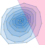
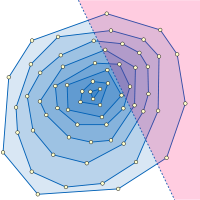
. For example, consider the problem of half-plane range reporting: that is, intersecting a fixed set of n points with a query half-plane and listing all the points in the intersection. The problem is to structure the points in such a way that a query of this type may be answered efficiently in terms of the intersection size h. One structure that can be used for this purpose is the convex layers of the input point set, a family of nested convex polygon
s consisting of the convex hull
of the point set and the recursively-constructed convex layers of the remaining points. Within a single layer, the points inside the query half-plane may be found by performing a binary search for the half-plane boundary line's slope among the sorted sequence of convex polygon edge slopes, leading to the polygon vertex that is inside the query half-plane and farthest from its boundary, and then sequentially searching along the polygon edges to find all other vertices inside the query half-plane. The whole half-plane range reporting problem may be solved by repeating this search procedure starting from the outermost layer and continuing inwards until reaching a layer that is disjoint from the query halfspace. Fractional cascading speeds up the successive binary searches among the sequences of polygon edge slopes in each layer, leading to a data structure for this problem with space O(n) and query time O(log n + h). The data structure may be constructed in time O(n log n) by an algorithm of Chazelle (1985). As in our example, this application involves binary searches in a linear sequence of lists (the nested sequence of the convex layers), so the catalog graph is just a path.
Another application of fractional cascading in geometric data structures concerns point location
in a monotone subdivision, that is, a partition of the plane into polygons such that any vertical line intersects any polygon in at most two points. As Edelsbrunner et al. (1986) showed, this problem can be solved by finding a sequence of polygonal paths that stretch from left to right across the subdivision, and binary searching for the lowest of these paths that is above the query point. Testing whether the query point is above or below one of the paths can itself be solved as a binary search problem, searching for the x coordinate of the points among the x coordinates of the path vertices to determine which path edge might be above or below the query point. Thus, each point location query can be solved as an outer layer of binary search among the paths, each step of which itself performs a binary search among x coordinates of vertices. Fractional cascading can be used to speed up the time for the inner binary searches, reducing the total time per query to O(log n) using a data structure with space O(n). In this application the catalog graph is a tree representing the possible search sequences of the outer binary search.
Beyond computational geometry, Lakshman and Stiliadis (1998) and Buddikot et al. (1999) apply fractional cascading in the design of data structures for fast packet filtering in internet routers. Gao et al. (2004) use fractional cascading as a model for data distribution and retrieval in sensor networks.
Computer science
Computer science or computing science is the study of the theoretical foundations of information and computation and of practical techniques for their implementation and application in computer systems...
, fractional cascading is a technique to speed up a sequence of binary searches for the same value in a sequence of related data structures. The first binary search in the sequence takes a logarithmic amount of time, as is standard for binary searches, but successive searches in the sequence are faster. The original version of fractional cascading, introduced in two papers by Chazelle
Bernard Chazelle
Bernard Chazelle is the Eugene Higgins Professor of Computer Science at Princeton University. Much of his work is in computational geometry, where he has found many of the best-known algorithms, such as linear-time triangulation of a simple polygon, as well as many useful complexity results, such...
and Guibas
Leonidas J. Guibas
Leonidas John Guibas is a professor of computer science at Stanford University, where he heads the geometric computation group and is a member of the computer graphics and artificial intelligence laboratories. Guibas was a student of Donald Knuth at Stanford, where he received his Ph.D. in 1976...
in 1986, combined the idea of cascading, originating in range searching
Range searching
In its most general form, the range searching problem consists of preprocessing a set S of objects, in order to determine which objects from S a query object, called a range, intersects...
data structures of and , with the idea of fractional sampling, which originated in . Later authors introduced more complex forms of fractional cascading that allow the data structure to be maintained as the data changes by a sequence of discrete insertion and deletion events.
Example
As a simple example of fractional cascading, consider the following problem. We are given as input a collection of k ordered lists Li of real numberReal number
In mathematics, a real number is a value that represents a quantity along a continuum, such as -5 , 4/3 , 8.6 , √2 and π...
s, such that the total length Σ|Li| of all lists is n, and must process them so that we can perform binary searches for a query value q in each of the k lists. For instance, with k = 4 and n = 17,
- L1 = 2.4, 6.4, 6.5, 8.0, 9.3
- L2 = 2.3, 2.5, 2.6
- L3 = 1.3, 4.4, 6.2, 6.6
- L4 = 1.1, 3.5, 4.6, 7.9, 8.1
The simplest solution to this searching problem is just to store each list separately. If we do so, the space requirement is O(n), but the time to perform a query is O(k log(n/k)), as we must perform a separate binary search in each of k lists. The worst case for querying this structure occurs when each of the k lists has equal size n/k, so each of the k binary searches involved in a query takes time O(log(n/k)).
A second solution allows faster queries at the expense of more space: we may merge all the k lists into a single big list L, and associate
with each item x of L a list of the results of searching for x in each of the smaller lists Li. If we describe an element of this merged list as x[a,b,c,d] where x is the numerical value and a, b, c, and d are the positions (the first number has position 0) of the next element at least as large as x in each of the original input lists (or the position after the end of the list if no such element exists), then we would have
- L = 1.1[0,0,0,0], 1.3[0,0,0,1], 2.3[0,0,1,1], 2.4[0,1,1,1], 2.5[1,1,1,1], 2.6[1,2,1,1],
- 3.5[1,3,1,1], 4.4[1,3,1,2], 4.6[1,3,2,2], 6.2[1,3,2,3], 6.4[1,3,3,3], 6.5[2,3,3,3],
- 6.6[3,3,3,3], 7.9[3,3,4,3], 8.0[3,3,4,4], 8.1[4,3,4,4], 9.3[4,3,4,5]
This merged solution allows a query in time O(log n + k): simply search for q in L and then report the results stored at the item x found by this search. For instance, if q = 5.0, searching for q in L finds the item 6.2[1,3,2,3], from which we return the results L1[1] = 6.4, L2[3] (a flag value indicating that q is past the end of L2), L3[2] = 6.2, and L4[3] = 7.9. However, this solution pays a high penalty in space complexity: it uses space O(kn) as each of the n items in L must store a list of k search results.
Fractional cascading allows this same searching problem to be solved with time and space bounds meeting the best of both worlds: query time O(log n + k), and space O(n).
The fractional cascading solution is to store a new sequence of lists Mi. The final list in this sequence, Mk, is equal to Lk; each earlier list Mi is formed by merging Li with every second item from Mi + 1. With each item x in this merged list, we store two numbers: the position resulting from searching for x in Li and the position resulting from searching for x in Mi + 1. For the data above, this would give us the following lists:
- M1 = 2.4[0, 1], 2.5[1, 1], 3.5[1, 3], 6.4[1, 5], 6.5[2, 5], 7.9[3, 5], 8[3, 6], 9.3[4, 6]
- M2 = 2.3[0, 1], 2.5[1, 1], 2.6[2, 1], 3.5[3, 1], 6.2[3, 3], 7.9[3, 5]
- M3 = 1.3[0, 1], 3.5[1, 1], 4.4[1, 2], 6.2[2, 3], 6.6[3, 3], 7.9[4, 3]
- M4 = 1.1[0, 0], 3.5[1, 0], 4.6[2, 0], 7.9[3, 0], 8.1[4, 0]
Suppose we wish to perform a query in this structure, for q = 5. We first do a standard binary search for q in M1, finding the value 6.4[1,5]. The "1" in 6.4[1,5], tells us that the search for q in L1 should return L1[1] = 6.4. The "5" in 6.4[1,5] tells us that the approximate location of q in M2 is position 5. More precisely, binary searching for q in M2 would return either the value 7.9[3, 5] at position 5, or the value 6.2[3, 3] one place earlier. By comparing q to 6.2, and observing that it is smaller, we determine that the correct search result in M2 is 6.2[3, 3]. The first "3" in 6.2[3, 3] tells us that the search for q in L2 should return L2[3], a flag value meaning that q is past the end of list L2. The second "3" in 6.2[3, 3] tells us that the approximate location of q in M3 is position 3. More precisely, binary searching for q in M3 would return either the value 6.2[2, 3] at position 3, or the value 4.4[1, 2] one place earlier. A comparison of q with the smaller value 4.4 shows us that the correct search result in M3 is 6.2[2,3]. The "2" in 6.2[2,3] tells us that the search for q in L3 should return L3[2] = 6.2, and the "3" in 6.2[2,3] tells us that the result of searching for q in M4 is either M4[3] = 7.9[3,0] or M4[2] = 4.6[0,0]; comparing q with 4.6 shows that the correct result is 7.9[3,0] and that the result of searching for q in L4 is L4[3] = 7.9. Thus, we have found q in each of our four lists, by doing a binary search in the single list M1 followed by a single comparison in each of the successive lists.
More generally, for any data structure of this type, we perform a query by doing a binary search for q in M1, and determining from the resulting value the position of q in L1. Then, for each i > 1, we use the known position of q in Mi to find its position in Mi + 1. The value associated with the position of q in Mi points to a position in Mi + 1 that is either the correct result of the binary search for q in Mi + 1 or is a single step away from that correct result, so stepping from i to i + 1 requires only a single comparison. Thus, the total time for a query is O(log n + k).
In our example, the fractionally cascaded lists have a total of 25 elements, less than twice that of the original input.
In general, the size of Mi in this data structure is at most
as may easily be proven by induction. Therefore, the total size of the data structure is at most
as may be seen by regrouping the contributions to the total size coming from the same input list Li together with each other.
The general problem
In general, fractional cascading begins with a catalog graph, a directed graphDirected graph
A directed graph or digraph is a pair G= of:* a set V, whose elements are called vertices or nodes,...
in which each vertex
Vertex (graph theory)
In graph theory, a vertex or node is the fundamental unit out of which graphs are formed: an undirected graph consists of a set of vertices and a set of edges , while a directed graph consists of a set of vertices and a set of arcs...
is labeled with an ordered list. A query in this data structure consists of a path
Path (graph theory)
In graph theory, a path in a graph is a sequence of vertices such that from each of its vertices there is an edge to the next vertex in the sequence. A path may be infinite, but a finite path always has a first vertex, called its start vertex, and a last vertex, called its end vertex. Both of them...
in the graph and a query value q; the data structure must determine the position of q in each of the ordered lists associated with the vertices of the path. For the simple example above, the catalog graph is itself a path, with just four nodes. It is possible for later vertices in the path to be determined dynamically as part of a query, in response to the results found by the searches in earlier parts of the path.
To handle queries of this type, for a graph in which each vertex has at most d incoming and at most d outgoing edges for some constant d, the lists associated with each vertex are augmented by a fraction of the items from each outgoing neighbor of the vertex; the fraction must be chosen to be smaller than 1/d, so that the total amount by which all lists are augmented remains linear in the input size. Each item in each augmented list stores with it the position of that item in the unaugmented list stored at the same vertex, and in each of the outgoing neighboring lists. In the simple example above, d = 1, and we augmented each list with a 1/2 fraction of the neighboring items.
A query in this data structure consists of a standard binary search in the augmented list associated with the first vertex of the query path, together with simpler searches at each successive vertex of the path. If a 1/r fraction of items are used to augment the lists from each neighboring item, then each successive query result may be found within at most r steps of the position stored at the query result from the previous path vertex, and therefore may be found in constant time without having to perform a full binary search.
Dynamic fractional cascading
In dynamic fractional cascading, the list stored at each node of the catalog graph may change dynamically, by a sequence of updates in which list items are inserted and deleted. This causes several difficulties for the data structure.First, when an item is inserted or deleted at a node of the catalog graph, it must be placed within the augmented list associated with that node, and may cause changes to propagate to other nodes of the catalog graph. Instead of storing the augmented lists in arrays, they should be stored as binary search trees, so that these changes can be handled efficiently while still allowing binary searches of the augmented lists.
Second, an insertion or deletion may cause a change to the subset of the list associated with a node that is passed on to neighboring nodes of the catalog graph. It is no longer feasible, in the dynamic setting, for this subset to be chosen as the items at every dth position of the list, for some d, as this subset would change too drastically after every update. Rather, a technique closely related to B-tree
B-tree
In computer science, a B-tree is a tree data structure that keeps data sorted and allows searches, sequential access, insertions, and deletions in logarithmic time. The B-tree is a generalization of a binary search tree in that a node can have more than two children...
s allows the selection of a fraction of data that is guaranteed to be smaller than 1/d, with the selected items guaranteed to be spaced a constant number of positions apart in the full list, and such that an insertion or deletion into the augmented list associated with a node causes changes to propagate to other nodes for a fraction of the operations that is less than 1/d. In this way, the distribution of the data among the nodes satisfies the properties needed for the query algorithm to be fast, while guaranteeing that the average number of binary search tree operations per data insertion or deletion is constant.
Third, and most critically, the static fractional cascading data structure maintains, for each element x of the augmented list at each node of the catalog graph, the index of the result that would be obtained when searching for x among the input items from that node and among the augmented lists stored at neighboring nodes. However, this information would be too expensive to maintain in the dynamic setting. Inserting or deleting a single value x could cause the indexes stored at an unbounded number of other values to change. Instead, dynamic versions of fractional cascading maintain several data structures for each node:
- A mapping of the items in the augmented list of the node to small integers, such that the ordering of the positions in the augmented list is equivalent to the comparison ordering of the integers, and a reverse map from these integers back to the list items. A technique of Dietz (1982) allows this numbering to be maintained efficiently.
- An integer searching data structure such as a van Emde Boas treeVan Emde Boas treeA van Emde Boas tree , also known as a vEB tree, is a tree data structure which implements an associative array with m-bit integer keys. It performs all operations in O time...
for the numbers associated with the input list of the node. With this structure, and the mapping from items to integers, one can efficiently find for each element x of the augmented list, the item that would be found on searching for x in the input list. - For each neighboring node in the catalog graph, a similar integer searching data structure for the numbers associated with the subset of the data propagated from the neighboring node. With this structure, and the mapping from items to integers, one can efficiently find for each element x of the augmented list, a position within a constant number of steps of the location of x in the augmented list associated with the neighboring node.
These data structures allow dynamic fractional cascading to be performed at a time of O(log n) per insertion or deletion, and a sequence of k binary searches following a path of length k in the catalog graph to be performed in time O(log n + k log log n).
Applications
Computational geometry
Computational geometry is a branch of computer science devoted to the study of algorithms which can be stated in terms of geometry. Some purely geometrical problems arise out of the study of computational geometric algorithms, and such problems are also considered to be part of computational...
. For example, consider the problem of half-plane range reporting: that is, intersecting a fixed set of n points with a query half-plane and listing all the points in the intersection. The problem is to structure the points in such a way that a query of this type may be answered efficiently in terms of the intersection size h. One structure that can be used for this purpose is the convex layers of the input point set, a family of nested convex polygon
Convex polygon
In geometry, a polygon can be either convex or concave .- Convex polygons :A convex polygon is a simple polygon whose interior is a convex set...
s consisting of the convex hull
Convex hull
In mathematics, the convex hull or convex envelope for a set of points X in a real vector space V is the minimal convex set containing X....
of the point set and the recursively-constructed convex layers of the remaining points. Within a single layer, the points inside the query half-plane may be found by performing a binary search for the half-plane boundary line's slope among the sorted sequence of convex polygon edge slopes, leading to the polygon vertex that is inside the query half-plane and farthest from its boundary, and then sequentially searching along the polygon edges to find all other vertices inside the query half-plane. The whole half-plane range reporting problem may be solved by repeating this search procedure starting from the outermost layer and continuing inwards until reaching a layer that is disjoint from the query halfspace. Fractional cascading speeds up the successive binary searches among the sequences of polygon edge slopes in each layer, leading to a data structure for this problem with space O(n) and query time O(log n + h). The data structure may be constructed in time O(n log n) by an algorithm of Chazelle (1985). As in our example, this application involves binary searches in a linear sequence of lists (the nested sequence of the convex layers), so the catalog graph is just a path.
Another application of fractional cascading in geometric data structures concerns point location
Point location
The point location problem is a fundamental topic of computational geometry. It finds applications in areas that deal with processing geometrical data: computer graphics, geographic information systems , motion planning, and computer aided design ....
in a monotone subdivision, that is, a partition of the plane into polygons such that any vertical line intersects any polygon in at most two points. As Edelsbrunner et al. (1986) showed, this problem can be solved by finding a sequence of polygonal paths that stretch from left to right across the subdivision, and binary searching for the lowest of these paths that is above the query point. Testing whether the query point is above or below one of the paths can itself be solved as a binary search problem, searching for the x coordinate of the points among the x coordinates of the path vertices to determine which path edge might be above or below the query point. Thus, each point location query can be solved as an outer layer of binary search among the paths, each step of which itself performs a binary search among x coordinates of vertices. Fractional cascading can be used to speed up the time for the inner binary searches, reducing the total time per query to O(log n) using a data structure with space O(n). In this application the catalog graph is a tree representing the possible search sequences of the outer binary search.
Beyond computational geometry, Lakshman and Stiliadis (1998) and Buddikot et al. (1999) apply fractional cascading in the design of data structures for fast packet filtering in internet routers. Gao et al. (2004) use fractional cascading as a model for data distribution and retrieval in sensor networks.
External links
- Lecture notes on fractional cascading from the University of North CarolinaUniversity of North Carolina at Chapel HillThe University of North Carolina at Chapel Hill is a public research university located in Chapel Hill, North Carolina, United States...
.