

Diffusion Monte Carlo
Encyclopedia
Diffusion Monte Carlo is a quantum Monte Carlo
method that uses a Green's function
to solve the Schrödinger equation
. DMC is potentially numerically exact, meaning that it can find the exact ground state energy within a given error for any quantum system. When actually attempting the calculation, one finds that for boson
s, the algorithm scales as a polynomial with the system size, but for fermion
s, DMC is exponentially scaling with the system size. This makes exact large-scale DMC simulations for fermions impossible; however, with a clever approximation known as fixed-node, very accurate results can be obtained. What follows is an explanation of the basic algorithm, how it works, why fermions cause a problem, and how the fixed-node approximation resolves this problem.
We can condense the notation a bit by writing it in terms of an operator equation, with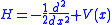 .
.
So then we have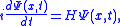
where we have to keep in mind that H
is an operator, not a simple number or function. There are special functions, called eigenfunction
s, for which , where E is a number. These functions are special because no matter where we evaluate the action of the H operator on the wave function, we always get the same number E. These functions are called stationary state
s, because the time derivative at any point x is always the same, so the amplitude of the wave function never changes in time. Since the overall phase of a wave function is not measurable, the system does not change in time.
We are usually interested in the wave function with the lowest energy
eigenvalue, the ground state
. We're going to write a slightly different version of the Schrödinger equation that will have the same energy eigenvalue, but, instead of being oscillatory, it will be convergent. Here it is: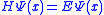 .
.
We've removed the imaginary number from the time derivative and added in a constant offset of , which is the ground state energy. We don't actually know the ground state energy, but there will be a way to determine it self-consistently which we'll introduce later. Our modified equation(some people call it the imaginary-time Schrödinger equation) has some nice properties. The first thing to notice is that if we happen to guess the ground state wave function, then
 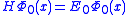 and the time derivative is zero. Now suppose that we start with another wave function(
 ), which is not the ground state but is not orthogonal to it. Then we can write it as a linear sum of eigenfunctions:
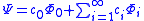
Since this is a linear differential equation
, we can look at the action of each part separately. We already determined that is stationary. Suppose we take
  . Since
  is the lowest-energy eigenfunction, the associate eigenvalue of
  satisfies the property
  . Thus the time derivative of
  is negative, and will eventually go to zero, leaving us with only the ground state. This observation also gives us a way to determine
  . We watch the amplitude of the wave function as we propagate through time. If it increases, then decrease the estimation of the offset energy. If the amplitude decreases, then increase the estimate of the offset energy.
 appropriately, we find the
ground state of any given Hamiltonian
. This is still a harder problem than classical mechanics
, though, because instead of
propagating single positions of particles, we must propagate entire functions. In classical mechanics, we could simulate the
motion of the particles by setting , if we assume that the force is constant over the time span of
  . For the imaginary time Schrödinger equation, instead, we propagate forward in time using a convolution
integral with a special function called a Green's function
. So we get . Similarly to classical mechanics, we can only propagate for small slices of time; otherwise the Green's function is inaccurate. As the number of particles increases, the dimensionality of the integral increases as well, since we have to integrate over all coordinates of all particles. We can do these integrals by Monte Carlo integration.
Quantum Monte Carlo
Quantum Monte Carlo is a large class of computer algorithms that simulate quantum systems with the idea of solving the quantum many-body problem. They use, in one way or another, the Monte Carlo method to handle the many-dimensional integrals that arise...
method that uses a Green's function
Green's function
In mathematics, a Green's function is a type of function used to solve inhomogeneous differential equations subject to specific initial conditions or boundary conditions...
to solve the Schrödinger equation
Schrödinger equation
The Schrödinger equation was formulated in 1926 by Austrian physicist Erwin Schrödinger. Used in physics , it is an equation that describes how the quantum state of a physical system changes in time....
. DMC is potentially numerically exact, meaning that it can find the exact ground state energy within a given error for any quantum system. When actually attempting the calculation, one finds that for boson
Boson
In particle physics, bosons are subatomic particles that obey Bose–Einstein statistics. Several bosons can occupy the same quantum state. The word boson derives from the name of Satyendra Nath Bose....
s, the algorithm scales as a polynomial with the system size, but for fermion
Fermion
In particle physics, a fermion is any particle which obeys the Fermi–Dirac statistics . Fermions contrast with bosons which obey Bose–Einstein statistics....
s, DMC is exponentially scaling with the system size. This makes exact large-scale DMC simulations for fermions impossible; however, with a clever approximation known as fixed-node, very accurate results can be obtained. What follows is an explanation of the basic algorithm, how it works, why fermions cause a problem, and how the fixed-node approximation resolves this problem.
The Projector Method
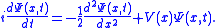
To motivate the algorithm, let's look at the Schrödinger equation for a particle in some potential in one dimension:We can condense the notation a bit by writing it in terms of an operator equation, with
.So then we have
where we have to keep in mind that H
Hamiltonian (quantum mechanics)
In quantum mechanics, the Hamiltonian H, also Ȟ or Ĥ, is the operator corresponding to the total energy of the system. Its spectrum is the set of possible outcomes when one measures the total energy of a system...
is an operator, not a simple number or function. There are special functions, called eigenfunction
Eigenfunction
In mathematics, an eigenfunction of a linear operator, A, defined on some function space is any non-zero function f in that space that returns from the operator exactly as is, except for a multiplicative scaling factor. More precisely, one has...
s, for which
, where E is a number. These functions are special because no matter where we evaluate the action of the H operator on the wave function, we always get the same number E. These functions are called stationary stateStationary state
In quantum mechanics, a stationary state is an eigenvector of the Hamiltonian, implying the probability density associated with the wavefunction is independent of time . This corresponds to a quantum state with a single definite energy...
s, because the time derivative at any point x is always the same, so the amplitude of the wave function never changes in time. Since the overall phase of a wave function is not measurable, the system does not change in time.
We are usually interested in the wave function with the lowest energy
Energy
In physics, energy is an indirectly observed quantity. It is often understood as the ability a physical system has to do work on other physical systems...
eigenvalue, the ground state
Ground state
The ground state of a quantum mechanical system is its lowest-energy state; the energy of the ground state is known as the zero-point energy of the system. An excited state is any state with energy greater than the ground state...
. We're going to write a slightly different version of the Schrödinger equation that will have the same energy eigenvalue, but, instead of being oscillatory, it will be convergent. Here it is:
.We've removed the imaginary number from the time derivative and added in a constant offset of
, which is the ground state energy. We don't actually know the ground state energy, but there will be a way to determine it self-consistently which we'll introduce later. Our modified equation(some people call it the imaginary-time Schrödinger equation) has some nice properties. The first thing to notice is that if we happen to guess the ground state wave function, then and the time derivative is zero. Now suppose that we start with another wave function(), which is not the ground state but is not orthogonal to it. Then we can write it as a linear sum of eigenfunctions:Since this is a linear differential equation
Linear differential equation
Linear differential equations are of the formwhere the differential operator L is a linear operator, y is the unknown function , and the right hand side ƒ is a given function of the same nature as y...
, we can look at the action of each part separately. We already determined that
is stationary. Suppose we take . Since is the lowest-energy eigenfunction, the associate eigenvalue of satisfies the property . Thus the time derivative of is negative, and will eventually go to zero, leaving us with only the ground state. This observation also gives us a way to determine . We watch the amplitude of the wave function as we propagate through time. If it increases, then decrease the estimation of the offset energy. If the amplitude decreases, then increase the estimate of the offset energy.Stochastic Implementation
Now we have an equation that, as we propagate it forward in time and adjust appropriately, we find theground state of any given Hamiltonian
Hamiltonian (quantum mechanics)
In quantum mechanics, the Hamiltonian H, also Ȟ or Ĥ, is the operator corresponding to the total energy of the system. Its spectrum is the set of possible outcomes when one measures the total energy of a system...
. This is still a harder problem than classical mechanics
Classical mechanics
In physics, classical mechanics is one of the two major sub-fields of mechanics, which is concerned with the set of physical laws describing the motion of bodies under the action of a system of forces...
, though, because instead of
propagating single positions of particles, we must propagate entire functions. In classical mechanics, we could simulate the
motion of the particles by setting
, if we assume that the force is constant over the time span of . For the imaginary time Schrödinger equation, instead, we propagate forward in time using a convolutionConvolution
In mathematics and, in particular, functional analysis, convolution is a mathematical operation on two functions f and g, producing a third function that is typically viewed as a modified version of one of the original functions. Convolution is similar to cross-correlation...
integral with a special function called a Green's function
Green's function
In mathematics, a Green's function is a type of function used to solve inhomogeneous differential equations subject to specific initial conditions or boundary conditions...
. So we get
. Similarly to classical mechanics, we can only propagate for small slices of time; otherwise the Green's function is inaccurate. As the number of particles increases, the dimensionality of the integral increases as well, since we have to integrate over all coordinates of all particles. We can do these integrals by Monte Carlo integration.