Ingrid Daubechies is a Belgian physicist and mathematician. She was between 2004 and 2011 the William R. Kenan Jr. Professor in the mathematics and applied mathematics departments at Princeton University. In January 2011 she moved to Duke University as a Professor in mathematics. She is the first...
An orthogonal wavelet is a wavelet where the associated wavelet transform is orthogonal.That is the inverse wavelet transform is the adjoint of the wavelet transform.If this condition is weakened you may end up with biorthogonal wavelets.- Basics :...
In numerical analysis and functional analysis, a discrete wavelet transform is any wavelet transform for which the wavelets are discretely sampled...
and characterized by a maximal number of vanishing moments
Moment (mathematics)
In mathematics, a moment is, loosely speaking, a quantitative measure of the shape of a set of points. The "second moment", for example, is widely used and measures the "width" of a set of points in one dimension or in higher dimensions measures the shape of a cloud of points as it could be fit by...
for some given support. With each wavelet type of this class, there is a scaling function (also called father wavelet) which generates an orthogonal multiresolution analysis.
Properties
In general the Daubechies wavelets are chosen to have the highest number A of vanishing moments, (this does not imply the best smoothness) for given support width N=2A, and among the 2A−1 possible solutions the one is chosen whose scaling filter has extremal phase. The wavelet transform is also easy to put into practice using the fast wavelet transform
Fast wavelet transform
The Fast Wavelet Transform is a mathematical algorithm designed to turn a waveform or signal in the time domain into a sequence of coefficients based on an orthogonal basis of small finite waves, or wavelets...
. Daubechies wavelets are widely used in solving a broad range of problems, e.g. self-similarity properties of a signal or fractal
Fractal
A fractal has been defined as "a rough or fragmented geometric shape that can be split into parts, each of which is a reduced-size copy of the whole," a property called self-similarity...
problems, signal discontinuities, etc.
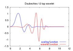
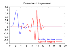
The Daubechies wavelets are not defined in terms of the resulting scaling and wavelet functions; in fact, they are not possible to write down in closed form. The graphs below are generated using the cascade algorithm
Cascade algorithm
In the mathematical topic of wavelet theory, the cascade algorithm is a numerical method for calculating function values of the basic scaling and wavelet functions of a discrete wavelet transform using an iterative algorithm. It starts from values on a coarse sequence of sampling points and...
, a numeric technique consisting of simply inverse-transforming [1 0 0 0 0 ... ] an appropriate number of times.
scaling and wavelet functions
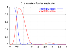
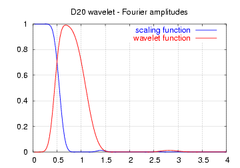
amplitudes of the frequency spectra of the above functions
Note that the spectra shown here are not the frequency response of the high and low pass filters, but rather the amplitudes of the continuous Fourier transforms of the scaling (blue) and wavelet (red) functions.
Daubechies orthogonal wavelets D2-D20 (even index numbers only) are commonly used. The index number refers to the number N of coefficients. Each wavelet has a number of zero moments or vanishing moments equal to half the number of coefficients. For example, D2 (the Haar wavelet
Haar wavelet
In mathematics, the Haar wavelet is a certain sequence of rescaled "square-shaped" functions which together form a wavelet family or basis. Wavelet analysis is similar to Fourier analysis in that it allows a target function over an interval to be represented in terms of an orthonormal function basis...
) has one vanishing moment, D4 has two, etc. A vanishing moment limits the wavelet's ability to represent polynomial
Polynomial
In mathematics, a polynomial is an expression of finite length constructed from variables and constants, using only the operations of addition, subtraction, multiplication, and non-negative integer exponents...
behaviour or information in a signal. For example, D2, with one moment, easily encodes polynomials of one coefficient, or constant signal components. D4 encodes polynomials with two coefficients, i.e. constant and linear signal components; and D6 encodes 3-polynomials, i.e. constant, linear and quadratic
Quadratic polynomial
In mathematics, a quadratic polynomial or quadratic is a polynomial of degree two, also called second-order polynomial. That means the exponents of the polynomial's variables are no larger than 2...
signal components. This ability to encode signals is nonetheless subject to the phenomenon of scale leakage, and the lack of shift-invariance, which arise from the discrete shifting operation (below) during application of the transform. Sub-sequences which represent linear, quadratic
Quadratic polynomial
In mathematics, a quadratic polynomial or quadratic is a polynomial of degree two, also called second-order polynomial. That means the exponents of the polynomial's variables are no larger than 2...
(for example) signal components are treated differently by the transform depending on whether the points align with even- or odd-numbered locations in the sequence. The lack of the important property of shift-invariance, has led to the development of several different versions of a shift-invariant (discrete) wavelet transform.
Construction
Both the scaling sequence (Low-Pass Filter) and the wavelet sequence (Band-Pass Filter) (see orthogonal wavelet
Orthogonal wavelet
An orthogonal wavelet is a wavelet where the associated wavelet transform is orthogonal.That is the inverse wavelet transform is the adjoint of the wavelet transform.If this condition is weakened you may end up with biorthogonal wavelets.- Basics :...
for details of this construction) will here be normalized to have sum equal 2 and sum of squares equal 2. In some applications, they are normalised to have sum , so that both sequences and all shifts of them by an even number of coefficients are orthonormal to each other.
Using the general representation for a scaling sequence of an orthogonal discrete wavelet transform with approximation order A,, with N=2A, p having real coefficients, p(1)=1 and degree(p)=A-1,
one can write the orthogonality condition as, or equally as (*),
with the Laurent-polynomial generating all symmetric sequences and . Further, P(X) stands for the symmetric Laurent-polynomial . Since and , P takes nonnegative values on the segment [0,2].
Equation (*) has one minimal solution for each A, which can be obtained by division in the ring
of truncated power series in X,.
Obviously, this has positive values on (0,2)
The homogeneous equation for (*) is antisymmetric about X=1 and has thus the general solution , with R some polynomial with real coefficients. That the sum
shall be nonnegative on the interval [0,2] translates into a set of linear restrictions on the coefficients of R. The values of P on the interval [0,2] are bounded by some quantity , maximizing r results in a linear program with infinitely many inequality conditions.
To solve for p one uses a technique called spectral factorization resp. Fejer-Riesz-algorithm. The polynomial P(X) splits into linear factors , N=A+1+2deg(R). Each linear factor represents a Laurent-polynomial that can be factored into two linear factors.
One can assign either one of the two linear factors to p(Z), thus one obtains 2N possible solutions. For extremal phase one chooses the one that has all complex roots of p(Z) inside or on the unit circle and is thus real.
The scaling sequences of lowest approximation order
Below are the coefficients for the scaling functions for D2-20. The wavelet coefficients are derived by reversing the order of the scaling function coefficients and then reversing the sign of every second one, (i.e., D4 wavelet = {-0.1830127, -0.3169873, 1.1830127, -0.6830127}). Mathematically, this looks like
where k is the coefficient index, b is a coefficient of the wavelet sequence and a a coefficient of the scaling sequence. N is the wavelet index, i.e., 2 for D2.
Parts of the construction are also used to derive the biorthogonal Cohen-Daubechies-Feauveau wavelet
Cohen-Daubechies-Feauveau wavelet
Cohen-Daubechies-Feauveau wavelet are the historically first family of biorthogonal wavelets, which was made popular by Ingrid Daubechies. These are not the same as the orthogonal Daubechies wavelets, and also not very similar in shape and properties...
Mathematica is a computational software program used in scientific, engineering, and mathematical fields and other areas of technical computing...
supports Daubechies wavelets directly a basic implementation is simple in MATLAB
MATLAB
MATLAB is a numerical computing environment and fourth-generation programming language. Developed by MathWorks, MATLAB allows matrix manipulations, plotting of functions and data, implementation of algorithms, creation of user interfaces, and interfacing with programs written in other languages,...
(in this case, Daubechies 4). This implementation uses periodization to handle the problem of finite length signals. Other, more sophisticated methods are available, but often it is not necessary to use these as it only affects the very ends of the transformed signal. The periodization is accomplished in the forward transform directly in MATLAB vector notation, and the inverse transform by using the circshift function:
Transform, D4
It is assumed that S, a column vector with an even number of elements, has been pre-defined as the signal to be analyzed.


 , so that both sequences and all shifts of them by an even number of coefficients are orthonormal to each other.
 , with N=2A, p having real coefficients, p(1)=1 and degree(p)=A-1,
 , or equally as
  (*),
(*), generating all symmetric sequences and
  . Further, P(X) stands for the symmetric Laurent-polynomial
  . Since
  and
and  , P takes nonnegative values on the segment [0,2].
 .
. , with R some polynomial with real coefficients. That the sum
 , maximizing r results in a linear program with infinitely many inequality conditions.
 for p one uses a technique called spectral factorization resp. Fejer-Riesz-algorithm. The polynomial P(X) splits into linear factors
  , N=A+1+2deg(R). Each linear factor represents a Laurent-polynomial
  that can be factored into two linear factors.