
Bresenham's line algorithm
Encyclopedia
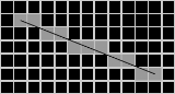
The Bresenham line algorithm is an algorithm
which determines which points in an n-dimensional raster
should be plotted in order to form a close approximation to a straight line between two given points. It is commonly used to draw lines on a computer screen, as it uses only integer addition, subtraction and bit shifting
, all of which are very cheap operations in standard computer architectures. It is one of the earliest algorithms developed in the field of computer graphics
. A minor extension to the original algorithm also deals with drawing circles.
While algorithms such as Wu's algorithm
are also frequently used in modern computer graphics because they can support antialiasing, the speed and simplicity of Bresenham's line algorithm mean that it is still important. The algorithm is used in hardware such as plotter
s and in the graphics chips
of modern graphics cards. It can also be found in many software graphics libraries
. Because the algorithm is very simple, it is often implemented in either the firmware
or the hardware
of modern graphics cards.
The label "Bresenham" is used today for a whole family of algorithms extending or modifying Bresenham's original algorithm. See further references below.
in 1962 at IBM. In 2001 Bresenham wrote:
Bresenham's algorithm was later modified to produce circles, the resulting algorithm being sometimes known as either "Bresenham's circle algorithm" or midpoint circle algorithm
.
 The common conventions will be used:
The endpoints of the line are the pixels at (x0, y0) and (x1, y1), where the first coordinate of the pair is the column and the second is the row.
The algorithm will be initially presented only for the octant
in which the segment goes down and to the right (x0≤x1 and y0≤y1), and its horizontal projection is longer than the vertical projection
  (the line has a slope
whose absolute value is less than 1 and greater than 0.)
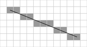
In this octant, for each column x between and
and  , there is exactly one row y (computed by the algorithm) containing a pixel of the line, while each row between
  and
and  may contain multiple rasterized pixels.
Bresenham's algorithm chooses the integer y corresponding to the pixel center that is closest to the ideal (fractional) y for the same x; on successive columns y can remain the same or increase by 1.
The general equation of the line through the endpoints is given by:
Since we know the column, x, the pixel's row, y, is given by rounding this quantity to the nearest integer:
The slope depends on the endpoint coordinates only and can be precomputed, and the ideal y for successive integer values of x can be computed starting from
  and repeatedly adding the slope.
In practice, the algorithm can track, instead of possibly large y values, a small error value between −0.5 and 0.5: the vertical distance between the rounded and the exact y values for the current x.
Each time x is increased, the error is increased by the slope; if it exceeds 0.5, the rasterization y is increased by 1 (the line continues on the next lower row of the raster) and the error is decremented by 1.0.
In the following pseudocode
sample
:
function line(x0, x1, y0, y1)
int deltax := x1 - x0
int deltay := y1 - y0
real error := 0
real deltaerr := abs (deltay / deltax) // Assume deltax != 0 (line is not vertical),
// note that this division needs to be done in a way that preserves the fractional part
int y := y0
for x from x0 to x1
plot(x,y)
error := error + deltaerr
if error ≥ 0.5 then
y := y + 1
error := error - 1.0
function line(x0, x1, y0, y1)
boolean steep := abs(y1 - y0) > abs(x1 - x0)
if steep then
swap(x0, y0)
swap(x1, y1)
if x0 > x1 then
swap(x0, x1)
swap(y0, y1)
int deltax := x1 - x0
int deltay := abs(y1 - y0)
real error := 0
real deltaerr := deltay / deltax
int ystep
int y := y0
if y0 < y1 then ystep := 1 else ystep := -1
for x from x0 to x1
if steep then plot(y,x) else plot(x,y)
error := error + deltaerr
if error ≥ 0.5 then
y := y + ystep
error := error - 1.0
The function now handles all lines and implements the complete Bresenham's algorithm.
function line(x0, x1, y0, y1)
boolean steep := abs(y1 - y0) > abs(x1 - x0)
if steep then
swap(x0, y0)
swap(x1, y1)
if x0 > x1 then
swap(x0, x1)
swap(y0, y1)
int deltax := x1 - x0
int deltay := abs(y1 - y0)
int error := deltax / 2
int ystep
int y := y0
if y0 < y1 then ystep := 1 else ystep := -1
for x from x0 to x1
if steep then plot(y,x) else plot(x,y)
error := error - deltay
if error < 0 then
y := y + ystep
error := error + deltax
Remark:
If you need to control the points in order of appearance (for example to print several consecutive dashed lines) you will have to simplify this code by skipping the 2nd swap:
function line(x0, x1, y0, y1)
boolean steep := abs(y1 - y0) > abs(x1 - x0)
if steep then
swap(x0, y0)
swap(x1, y1)
int deltax := abs(x1 - x0)
int deltay := abs(y1 - y0)
int error := deltax / 2
int ystep
int y := y0
int inc REM added
if x0 < x1 then inc := 1 else inc := -1 REM added
if y0 < y1 then ystep := 1 else ystep := -1
for x from x0 to x1 with increment inc REM changed
if steep then plot(y,x) else plot(x,y)
REM increment here a variable to control the progress of the line drawing
error := error - deltay
if error < 0 then
y := y + ystep
error := error + deltax
function line(x0, y0, x1, y1)
dx := abs(x1-x0)
dy := abs(y1-y0)
if x0 < x1 then sx := 1 else sx := -1
if y0 < y1 then sy := 1 else sy := -1
err := dx-dy
loop
setPixel(x0,y0)
if x0 = x1 and y0 = y1 exit loop
e2 := 2*err
if e2 > -dy then
err := err - dy
x0 := x0 + sx
end if
if e2 < dx then
err := err + dx
y0 := y0 + sy
end if
end loop
where m is the slope and b is the y-intercept. This is a function of only x and it would be useful to make this equation written as a function of both x and y. Using algebraic manipulation and recognition that the slope is the "rise over run" or then
then
Letting this last equation be a function of x and y then it can be written as

where the constants are
The line is then defined for some constants A, B, and C and anywhere . For any
  not on the line then
  . It should be noted that everything about this form involves only integers if x and y are integers since the constants are necessarily integers.
As an example, the line then this could be written as
  . The point (2,2) is on the line

and the point (2,3) is not on the line

and neither is the point (2,1)

Notice that the points (2,1) and (2,3) are on opposite sides of the line and f(x,y) evaluates to positive or negative. A line splits a plane into halves and the half-plane that has a negative f(x,y) can be called the negative half-plane, and the other half can called the positive half-plane. This observation is very important in the remainder of the derivation.

only because the line is defined to start and end on integer coordinates (though it's entirely reasonable to want to draw a line with non-integer end points).
Keeping in mind that the slope is less-than-or-equal-to one, the problem now presents itself as to whether the next point should be at or
or  . Perhaps intuitively, the point should be chosen based upon which is closer to the line at
  . If it is closer to the former then include the former point on the line, if the latter then the latter. To answer this, consider the midpoint between these two points:
If the value of this is negative then the midpoint lies above the line, and if the value of this is positive then the midpoint lies below the line. If the midpoint lies below the line then should be chosen since it is closer; otherwise
  should be chosen. This observation is crucial to understand! The value of the line function at this midpoint is the sole determinant of which point should be chosen.
The image to the right shows the blue point (2,2) chosen to be on the line with two candiate points in green (3,2) and (3,3). The black point (3, 2.5) is the midpoint between the two candiate points.
Alternatively, the difference between points can be used instead of evaluating f(x,y) at midpoints. The difference for the first decision is
If this difference, D, is positive then chose otherwise
  .
.
The decision for the second point can be written as


If the difference is positive then is chosen, otherwise
  . This decision can be generalized by accumulating the error.
All of the derivation for the algorithm is done. One performance issue is the 1/2 factor in the initial value of D. Since all of this is about the sign of the accumulated difference, then everything can be multiplied by 2 with no consequence.
This results in an algorithm that uses only integer arithmetic.
plot(x0,y0, x1,y1)
dx=x1-x0
dy=y1-y0
D = 2*dy - dx
plot(x0,y0)
y=y0
for x from x0+1 to x1
if D > 0
y = y+1
plot(x,y)
D = D + (2*dy-2*dx)
else
plot(x,y)
D = D + (2*dy)
Running this algorithm for from (0,1) to (6,4) yields the following differences with dx=6 and dy=3:
The result of this plot is shown to the right. The plotting can be viewed by plotting at the intersection of lines (blue circles) or filling in pixel boxes (yellow squares). Regardless, the plotting is the same.
. This means there are eight possible cases to consider.
(using 0.5 as error threshold instead of 0, which is required for non-overlapping polygon rasterizing).
The principle of using an incremental error in place of division operations has other applications in graphics. It is possible to use this technique to calculate the U,V co-ordinates
during raster scan of texture mapped polygons. The voxel
heightmap software-rendering engines seen in some PC games also used this principle.
Bresenham also published a Run-Slice (as opposed to the Run-Length) computational algorithm.
An extension to the algorithm that handles thick lines was created by Alan Murphy at IBM.
Algorithm
In mathematics and computer science, an algorithm is an effective method expressed as a finite list of well-defined instructions for calculating a function. Algorithms are used for calculation, data processing, and automated reasoning...
which determines which points in an n-dimensional raster
Raster graphics
In computer graphics, a raster graphics image, or bitmap, is a data structure representing a generally rectangular grid of pixels, or points of color, viewable via a monitor, paper, or other display medium...
should be plotted in order to form a close approximation to a straight line between two given points. It is commonly used to draw lines on a computer screen, as it uses only integer addition, subtraction and bit shifting
Bitwise operation
A bitwise operation operates on one or more bit patterns or binary numerals at the level of their individual bits. This is used directly at the digital hardware level as well as in microcode, machine code and certain kinds of high level languages...
, all of which are very cheap operations in standard computer architectures. It is one of the earliest algorithms developed in the field of computer graphics
Computer graphics
Computer graphics are graphics created using computers and, more generally, the representation and manipulation of image data by a computer with help from specialized software and hardware....
. A minor extension to the original algorithm also deals with drawing circles.
While algorithms such as Wu's algorithm
Xiaolin Wu's line algorithm
Xiaolin Wu's line algorithm is an algorithm for line antialiasing, which was presented in the article An Efficient Antialiasing Technique in the July 1991 issue of Computer Graphics, as well as in the article Fast Antialiasing in the June 1992 issue of Dr. Dobb's Journal.Bresenham's algorithm draws...
are also frequently used in modern computer graphics because they can support antialiasing, the speed and simplicity of Bresenham's line algorithm mean that it is still important. The algorithm is used in hardware such as plotter
Plotter
A plotter is a computer printing device for printing vector graphics. In the past, plotters were widely used in applications such as computer-aided design, though they have generally been replaced with wide-format conventional printers...
s and in the graphics chips
Graphics processing unit
A graphics processing unit or GPU is a specialized circuit designed to rapidly manipulate and alter memory in such a way so as to accelerate the building of images in a frame buffer intended for output to a display...
of modern graphics cards. It can also be found in many software graphics libraries
Graphics library
A graphics library is a program library designed to aid in rendering computer graphics to a monitor. This typically involves providing optimized versions of functions that handle common rendering tasks. This can be done purely in software and running on the CPU, common in embedded systems, or being...
. Because the algorithm is very simple, it is often implemented in either the firmware
Firmware
In electronic systems and computing, firmware is a term often used to denote the fixed, usually rather small, programs and/or data structures that internally control various electronic devices...
or the hardware
Hardware
Hardware is a general term for equipment such as keys, locks, hinges, latches, handles, wire, chains, plumbing supplies, tools, utensils, cutlery and machine parts. Household hardware is typically sold in hardware stores....
of modern graphics cards.
The label "Bresenham" is used today for a whole family of algorithms extending or modifying Bresenham's original algorithm. See further references below.
History
The algorithm was developed by Jack E. BresenhamJack E. Bresenham
Jack Elton Bresenham is a former professor of computer science.-Biography:He retired from 27 years of service at IBM as a Senior Technical Staff Member in 1987. He taught for 16 years at Winthrop University and has nine patents...
in 1962 at IBM. In 2001 Bresenham wrote:
I was working in the computation lab at IBM's San Jose development lab. A Calcomp plotterCalcomp plotterThe Calcomp 560 drum plotter, introduced in 1959, was one of the first computer graphics output devices sold. The computer could control in 0.01 inch increments the rotation of an 11 inch wide drum and the horizontal movement of a pen holder over the drum. A solenoid could press the pen against...
had been attached to an IBM 1401IBM 1401The IBM 1401 was a variable wordlength decimal computer that was announced by IBM on October 5, 1959. The first member of the highly successful IBM 1400 series, it was aimed at replacing electromechanical unit record equipment for processing data stored on punched cards...
via the 1407 typewriter console. [The algorithm] was in production use by summer 1962, possibly a month or so earlier. Programs in those days were freely exchanged among corporations so Calcomp (Jim Newland and Calvin Hefte) had copies. When I returned to Stanford in Fall 1962, I put a copy in the Stanford comp center library.
A description of the line drawing routine was accepted for presentation at the 1963 ACMAssociation for Computing MachineryThe Association for Computing Machinery is a learned society for computing. It was founded in 1947 as the world's first scientific and educational computing society. Its membership is more than 92,000 as of 2009...
national convention in Denver, Colorado. It was a year in which no proceedings were published, only the agenda of speakers and topics in an issue of Communications of the ACM. A person from the IBM Systems Journal asked me after I made my presentation if they could publish the paper. I happily agreed, and they printed it in 1965.
Bresenham's algorithm was later modified to produce circles, the resulting algorithm being sometimes known as either "Bresenham's circle algorithm" or midpoint circle algorithm
Midpoint circle algorithm
In computer graphics, the midpoint circle algorithm is an algorithm used to determine the points needed for drawing a circle. The algorithm is a variant of Bresenham's line algorithm, and is thus sometimes known as Bresenham's circle algorithm, although not actually invented by Bresenham...
.
The algorithm
- the top-left is (0,0) such that pixel coordinates increase in the right and down directions (e.g. that the pixel at (1,1) is directly above the pixel at (1,2)), and
- that the pixel centers have integer coordinates.
The endpoints of the line are the pixels at (x0, y0) and (x1, y1), where the first coordinate of the pair is the column and the second is the row.
The algorithm will be initially presented only for the octant
Octant
An octant is one of eight divisions.-Octant in the plane :Traditionally wind direction is given as one of the 8 octants because that is more accurate than merely giving one of the 4 quadrants, and the wind vane typically does not have enough accuracy to bother with more precise indication.-Octant...
in which the segment goes down and to the right (x0≤x1 and y0≤y1), and its horizontal projection
is longer than the vertical projection (the line has a slopeSlope
In mathematics, the slope or gradient of a line describes its steepness, incline, or grade. A higher slope value indicates a steeper incline....
whose absolute value is less than 1 and greater than 0.)
In this octant, for each column x between
and , there is exactly one row y (computed by the algorithm) containing a pixel of the line, while each row between and may contain multiple rasterized pixels.Bresenham's algorithm chooses the integer y corresponding to the pixel center that is closest to the ideal (fractional) y for the same x; on successive columns y can remain the same or increase by 1.
The general equation of the line through the endpoints is given by:
Since we know the column, x, the pixel's row, y, is given by rounding this quantity to the nearest integer:
The slope
depends on the endpoint coordinates only and can be precomputed, and the ideal y for successive integer values of x can be computed starting from and repeatedly adding the slope.In practice, the algorithm can track, instead of possibly large y values, a small error value between −0.5 and 0.5: the vertical distance between the rounded and the exact y values for the current x.
Each time x is increased, the error is increased by the slope; if it exceeds 0.5, the rasterization y is increased by 1 (the line continues on the next lower row of the raster) and the error is decremented by 1.0.
In the following pseudocode
Pseudocode
In computer science and numerical computation, pseudocode is a compact and informal high-level description of the operating principle of a computer program or other algorithm. It uses the structural conventions of a programming language, but is intended for human reading rather than machine reading...
sample
plot(x,y) plots a point and abs returns absolute valueAbsolute value
In mathematics, the absolute value |a| of a real number a is the numerical value of a without regard to its sign. So, for example, the absolute value of 3 is 3, and the absolute value of -3 is also 3...
:
function line(x0, x1, y0, y1)
int deltax := x1 - x0
int deltay := y1 - y0
real error := 0
real deltaerr := abs (deltay / deltax) // Assume deltax != 0 (line is not vertical),
// note that this division needs to be done in a way that preserves the fractional part
int y := y0
for x from x0 to x1
plot(x,y)
error := error + deltaerr
if error ≥ 0.5 then
y := y + 1
error := error - 1.0
Generalization
The version above only handles lines that descend to the right. We would of course like to be able to draw all lines. The first case is allowing us to draw lines that still slope downwards but head in the opposite direction. This is a simple matter of swapping the initial points ifx0 > x1. Trickier is determining how to draw lines that go up. To do this, we check if y0 ≥ y1; if so, we step y by -1 instead of 1. Lastly, we still need to generalize the algorithm to drawing lines in all directions. Up until now we have only been able to draw lines with a slope less than one. To be able to draw lines with a steeper slope, we take advantage of the fact that a steep line can be reflected across the line y=x to obtain a line with a small slope. The effect is to switch the x and y variables throughout, including switching the parameters to plot. The code looks like this:function line(x0, x1, y0, y1)
boolean steep := abs(y1 - y0) > abs(x1 - x0)
if steep then
swap(x0, y0)
swap(x1, y1)
if x0 > x1 then
swap(x0, x1)
swap(y0, y1)
int deltax := x1 - x0
int deltay := abs(y1 - y0)
real error := 0
real deltaerr := deltay / deltax
int ystep
int y := y0
if y0 < y1 then ystep := 1 else ystep := -1
for x from x0 to x1
if steep then plot(y,x) else plot(x,y)
error := error + deltaerr
if error ≥ 0.5 then
y := y + ystep
error := error - 1.0
The function now handles all lines and implements the complete Bresenham's algorithm.
Optimization
The problem with this approach is that computers operate relatively slowly on fractional numbers likeerror and deltaerr; moreover, errors can accumulate over many floating-point additions. Working with integers will be both faster and more accurate. The trick we use is to multiply all the fractional numbers (including the constant 0.5) in the code above by deltax, which enables us to express them as integers. This results in a divide inside the main loop, however. To deal with this we modify how error is initialized and used so that rather than starting at zero and counting up towards 0.5, it starts at 0.5 and counts down to zero. The new program looks like this:function line(x0, x1, y0, y1)
boolean steep := abs(y1 - y0) > abs(x1 - x0)
if steep then
swap(x0, y0)
swap(x1, y1)
if x0 > x1 then
swap(x0, x1)
swap(y0, y1)
int deltax := x1 - x0
int deltay := abs(y1 - y0)
int error := deltax / 2
int ystep
int y := y0
if y0 < y1 then ystep := 1 else ystep := -1
for x from x0 to x1
if steep then plot(y,x) else plot(x,y)
error := error - deltay
if error < 0 then
y := y + ystep
error := error + deltax
Remark:
If you need to control the points in order of appearance (for example to print several consecutive dashed lines) you will have to simplify this code by skipping the 2nd swap:
function line(x0, x1, y0, y1)
boolean steep := abs(y1 - y0) > abs(x1 - x0)
if steep then
swap(x0, y0)
swap(x1, y1)
int deltax := abs(x1 - x0)
int deltay := abs(y1 - y0)
int error := deltax / 2
int ystep
int y := y0
int inc REM added
if x0 < x1 then inc := 1 else inc := -1 REM added
if y0 < y1 then ystep := 1 else ystep := -1
for x from x0 to x1 with increment inc REM changed
if steep then plot(y,x) else plot(x,y)
REM increment here a variable to control the progress of the line drawing
error := error - deltay
if error < 0 then
y := y + ystep
error := error + deltax
Simplification
It is further possible to eliminate theswaps in the initialisation by considering the error calculation for both directions simultaneously:function line(x0, y0, x1, y1)
dx := abs(x1-x0)
dy := abs(y1-y0)
if x0 < x1 then sx := 1 else sx := -1
if y0 < y1 then sy := 1 else sy := -1
err := dx-dy
loop
setPixel(x0,y0)
if x0 = x1 and y0 = y1 exit loop
e2 := 2*err
if e2 > -dy then
err := err - dy
x0 := x0 + sx
end if
if e2 < dx then
err := err + dx
y0 := y0 + sy
end if
end loop
Derivation
To derive Bresenham's algorithm, two steps must be taken. The first step is transforming the equation of a line from the typical slope-intercept form into something different; and then using this new equation for a line to draw a line based on the idea of accumulation of error.Line equation
The slope-intercept form of a line is written aswhere m is the slope and b is the y-intercept. This is a function of only x and it would be useful to make this equation written as a function of both x and y. Using algebraic manipulation and recognition that the slope is the "rise over run" or
thenLetting this last equation be a function of x and y then it can be written as
where the constants are


The line is then defined for some constants A, B, and C and anywhere
. For any not on the line then . It should be noted that everything about this form involves only integers if x and y are integers since the constants are necessarily integers.As an example, the line
then this could be written as . The point (2,2) is on the lineand the point (2,3) is not on the line
and neither is the point (2,1)
Notice that the points (2,1) and (2,3) are on opposite sides of the line and f(x,y) evaluates to positive or negative. A line splits a plane into halves and the half-plane that has a negative f(x,y) can be called the negative half-plane, and the other half can called the positive half-plane. This observation is very important in the remainder of the derivation.
Algorithm
Clearly, the starting point is on the lineonly because the line is defined to start and end on integer coordinates (though it's entirely reasonable to want to draw a line with non-integer end points).
Keeping in mind that the slope is less-than-or-equal-to one, the problem now presents itself as to whether the next point should be at
or . Perhaps intuitively, the point should be chosen based upon which is closer to the line at . If it is closer to the former then include the former point on the line, if the latter then the latter. To answer this, consider the midpoint between these two points:If the value of this is negative then the midpoint lies above the line, and if the value of this is positive then the midpoint lies below the line. If the midpoint lies below the line then
should be chosen since it is closer; otherwise should be chosen. This observation is crucial to understand! The value of the line function at this midpoint is the sole determinant of which point should be chosen.The image to the right shows the blue point (2,2) chosen to be on the line with two candiate points in green (3,2) and (3,3). The black point (3, 2.5) is the midpoint between the two candiate points.
Alternatively, the difference between points can be used instead of evaluating f(x,y) at midpoints. The difference for the first decision is
If this difference, D, is positive then chose
otherwise .The decision for the second point can be written as
If the difference is positive then
is chosen, otherwise . This decision can be generalized by accumulating the error.All of the derivation for the algorithm is done. One performance issue is the 1/2 factor in the initial value of D. Since all of this is about the sign of the accumulated difference, then everything can be multiplied by 2 with no consequence.
This results in an algorithm that uses only integer arithmetic.
plot(x0,y0, x1,y1)
dx=x1-x0
dy=y1-y0
D = 2*dy - dx
plot(x0,y0)
y=y0
for x from x0+1 to x1
if D > 0
y = y+1
plot(x,y)
D = D + (2*dy-2*dx)
else
plot(x,y)
D = D + (2*dy)
Running this algorithm for
from (0,1) to (6,4) yields the following differences with dx=6 and dy=3:
- D=2*3-6=0
- plot(0,1)
- Loop from 1 to 6
- x=1: D≤0: plot(1,1), D=6
- x=2: D>0: y=2, plot(2,2), D=6+(6-12)=0
- x=3: D≤0: plot(3,2), D=6
- x=4: D>0: y=3, plot(4,3), D=6+(6-12)=0
- x=5: D≤0: plot(5,3), D=6
- x=6: D>0: y=4, plot(6,4), D=6+(6-12)=0
The result of this plot is shown to the right. The plotting can be viewed by plotting at the intersection of lines (blue circles) or filling in pixel boxes (yellow squares). Regardless, the plotting is the same.
All cases
However, as mentioned above this is only for the first octantOctant
An octant is one of eight divisions.-Octant in the plane :Traditionally wind direction is given as one of the 8 octants because that is more accurate than merely giving one of the 4 quadrants, and the wind vane typically does not have enough accuracy to bother with more precise indication.-Octant...
. This means there are eight possible cases to consider.
Similar algorithms
The Bresenham algorithm can be interpreted as slightly modified DDADigital Differential Analyzer (graphics algorithm)
In computer graphics, a hardware or software implementation of a digital differential analyzer is used for linear interpolation of variables over an interval between start and end point. DDAs are used for rasterization of lines, triangles and polygons...
(using 0.5 as error threshold instead of 0, which is required for non-overlapping polygon rasterizing).
The principle of using an incremental error in place of division operations has other applications in graphics. It is possible to use this technique to calculate the U,V co-ordinates
UV mapping
UV mapping is the 3D modeling process of making a 2D image representation of a 3D model.-UV mapping:This process projects a texture map onto a 3D object...
during raster scan of texture mapped polygons. The voxel
Voxel
A voxel is a volume element, representing a value on a regular grid in three dimensional space. This is analogous to a pixel, which represents 2D image data in a bitmap...
heightmap software-rendering engines seen in some PC games also used this principle.
Bresenham also published a Run-Slice (as opposed to the Run-Length) computational algorithm.
An extension to the algorithm that handles thick lines was created by Alan Murphy at IBM.
See also
- Digital Differential Analyzer (graphics algorithm)Digital Differential Analyzer (graphics algorithm)In computer graphics, a hardware or software implementation of a digital differential analyzer is used for linear interpolation of variables over an interval between start and end point. DDAs are used for rasterization of lines, triangles and polygons...
, a simple and general method for rasterizing lines and triangles - Xiaolin Wu's line algorithmXiaolin Wu's line algorithmXiaolin Wu's line algorithm is an algorithm for line antialiasing, which was presented in the article An Efficient Antialiasing Technique in the July 1991 issue of Computer Graphics, as well as in the article Fast Antialiasing in the June 1992 issue of Dr. Dobb's Journal.Bresenham's algorithm draws...
, a similarly fast method of drawing lines with antialiasing - Midpoint circle algorithmMidpoint circle algorithmIn computer graphics, the midpoint circle algorithm is an algorithm used to determine the points needed for drawing a circle. The algorithm is a variant of Bresenham's line algorithm, and is thus sometimes known as Bresenham's circle algorithm, although not actually invented by Bresenham...
, a similar algorithm for drawing circles
Further reading
- Patrick-Gilles Maillot's Thesis an extension of the Bresenham line drawing algorithm to perform 3D hidden lines removal; also published in MICAD '87 proceedings on CAD/CAM and Computer Graphics, page 591 - ISBN 2-86601-084-1.
- Line Thickening by Modification To Bresenham's Algorithm, A.S. Murphy, IBM Technical Disclosure Bulletin, Vol. 20, No. 12, May 1978.
External links
- Didactical Javascript implementation
- Analyze Bresenham's line algorithm in an online Javascript IDE
- The Bresenham Line-Drawing Algorithm by Colin Flanagan
- National Institute of Standards and Technology page on Bresenham's algorithm
- Calcomp 563 Incremental Plotter Information
- 3D extension
- Bresenham 2D, 3D up to 6D
- Bresenham Algorithm in several programming languages
- The Beauty of Bresenham's Algorithm – A simple implementation to plot lines, circles, ellipses and Bézier curves