
Arithmetic coding
Encyclopedia
Arithmetic coding is a form of variable-length
entropy encoding
used in lossless data compression
. Normally, a string of characters such as the words "hello there" is represented using a fixed number of bits per character, as in the ASCII code. When a string is converted to arithmetic encoding, frequently used characters will be stored with fewer bits and not-so-frequently occurring characters will be stored with more bits, resulting in fewer bits used in total. Arithmetic coding differs from other forms of entropy encoding such as Huffman coding
in that rather than separating the input into component symbols and replacing each with a code, arithmetic coding encodes the entire message into a single number, a fraction n where (0.0 ≤ n < 1.0).
A more efficient solution is to represent the sequence as a rational number between 0 and 1 in base 3, where each digit represents a symbol. For example, the sequence "ABBCAB" could become 0.0112013. The next step is to encode this ternary
number using a fixed-point binary number of sufficient precision to recover it, such as 0.0010110012 — this is only 9 bits, 25% smaller than the naïve block encoding. This is feasible for long sequences because there are efficient, in-place algorithms for converting the base of arbitrarily precise numbers.
To decode the value, knowing the original string had length 6, one can simply convert back to base 3, round to 6 digits, and recover the string.
Example: a simple, static model for describing the output of a particular monitoring instrument over time might be:
Models can also handle alphabets other than the simple four-symbol set chosen for this example. More sophisticated models are also possible: higher-order modelling changes its estimation of the current probability of a symbol based on the symbols that precede it (the context), so that in a model for English text, for example, the percentage chance of "u" would be much higher when it follows a "Q" or a "q". Models can even be adaptive
, so that they continuously change their prediction of the data based on what the stream actually contains. The decoder must have the same model as the encoder.
The encoder divides the current interval into sub-intervals, each representing a fraction of the current interval proportional to the probability of that symbol in the current context. Whichever interval corresponds to the actual symbol that is next to be encoded becomes the interval used in the next step.
Example: for the four-symbol model above:
When all symbols have been encoded, the resulting interval unambiguously identifies the sequence of symbols that produced it. Anyone who has the same final interval and model that is being used can reconstruct the symbol sequence that must have entered the encoder to result in that final interval.
It is not necessary to transmit the final interval, however; it is only necessary to transmit one fraction that lies within that interval. In particular, it is only necessary to transmit enough digits (in whatever base) of the fraction so that all fractions that begin with those digits fall into the final interval.
 Consider the process for decoding a message encoded with the given four-symbol model. The message is encoded in the fraction 0.538 (using decimal for clarity, instead of binary; also assuming that there are only as many digits as needed to decode the message.)
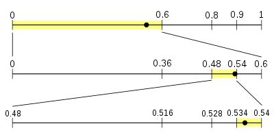
The process starts with the same interval used by the encoder:[0,1) , and using the same model, dividing it into the same four sub-intervals that the encoder must have. The fraction 0.538 falls into the sub-interval for NEUTRAL, [0, 0.6) ; this indicates that the first symbol the encoder read must have been NEUTRAL, so this is the first symbol of the message.
Next divide the interval[0, 0.6) into sub-intervals:
Since .538 is within the interval[0.48, 0.54) , the second symbol of the message must have been NEGATIVE.
Again divide our current interval into sub-intervals:
Now .538 falls within the interval of the END-OF-DATA symbol; therefore, this must be the next symbol. Since it is also the internal termination symbol, it means the decoding is complete. If the stream is not internally terminated, there needs to be some other way to indicate where the stream stops. Otherwise, the decoding process could continue forever, mistakenly reading more symbols from the fraction than were in fact encoded into it.
s; the same message could have been encoded in the binary fraction 0.10001010 (equivalent to 0.5390625 decimal) at a cost of only 8 bits. (The final zero must be specified in the binary fraction, or else the message would be ambiguous without external information such as compressed stream size.)
This 8 bit output is larger than the information content, or entropy
of the message, which is 1.57 × 3 or 4.71 bits. The large difference between the example's 8 (or 7 with external compressed data size information) bits of output and the entropy of 4.71 bits is caused by the short example message not being able to exercise the coder effectively. The claimed symbol probabilities were[0.6, 0.2, 0.1, 0.1] , but the actual frequencies in this example are [0.33, 0, 0.33, 0.33] . If the intervals are readjusted for these frequencies, the entropy of the message would be 1.58 bits and the same NEUTRAL NEGATIVE ENDOFDATA message could be encoded as intervals [0, 1/3); [1/9, 2/9); [5/27, 6/27); and a binary interval of [1011110, 1110001) . This could yield an output message of 111, or just 3 bits. This is also an example of how statistical coding methods like arithmetic encoding can produce an output message that is larger than the input message, especially if the probability model is off.
, and only converted the fraction to its final form at the end of encoding. Rather than try to simulate infinite precision, most arithmetic coders instead operate at a fixed limit of precision which they know the decoder will be able to match, and round the calculated fractions to their nearest equivalents at that precision. An example shows how this would work if the model called for the interval[0,1) to be divided into thirds, and this was approximated with 8 bit precision. Note that since now the precision is known, so are the binary ranges we'll be able to use.
A process called renormalization keeps the finite precision from becoming a limit on the total number of symbols that can be encoded. Whenever the range is reduced to the point where all values in the range share certain beginning digits, those digits are sent to the output. For however many digits of precision the computer can handle, it is now handling fewer than that, so the existing digits are shifted left, and at the right, new digits are added to expand the range as widely as possible. Note that this result occurs in two of the three cases from our previous example.
. For example, the following We may look at any sequence of symbols:

as a number in a certain base presuming that the involved symbols form an ordered set and each symbol in the ordered set denotes a sequential integer A = 0, B = 1, C = 2, D = 3, and so on. This results in the following frequencies and cumulative frequencies:
The cumulative frequency is the total of all frequencies below it in a frequency distribution (a running total of frequencies).
In a positional numeral system
the radix, or base, is numerically equal to a number of different symbols used to express the number. For example, in the decimal system the number of symbols is 10, namely 0,1,2,3,4,5,6,7,8,9. The radix is used to express any finite integer in a presumed multiplier in polynomial form. For example, the number 457 is actually 4×10² + 5×101 + 7×100, where base 10 is presumed but not shown explicitly.
Initially, we will convert DABDDB into a base-6 numeral, because 6 is the length of the string. The string is first mapped into the digit string 301331, which then maps to an integer by the polynomial:

The result 23671 has a length of 15 bits, which is not very close to the theoretical limit (the entropy of the message), which is approximately 9 bits.
To encode a message with a length closer to the theoretical limit imposed by information theory we need to slightly generalize the classic formula for changing the radix. We will compute lower and upper bounds L and U and choose a number between them. For the computation of L we multiply each term in the above expression by the product of the frequencies of all previously occurred symbols:

The difference between this polynomial and the polynomial above is that each term is multiplied by the product of the frequencies of all previously occurring symbols. More generally, L may be computed as:
where are the cumulative frequencies and
  are the frequencies of occurrences. Indexes denote the position of the symbol in a message. In the special case where all frequencies
  are 1, this is the change-of-base formula.
The upper bound U will be L plus the product of all frequencies; in this case U = L + (3 × 1 × 2 × 3 × 3 × 2) = 25002 + 108 = 25110. In general, U is given by:
Now we can choose any number from the interval [L, U) to represent the message; one convenient choice is the value with the longest possible trail of zeroes, 25100, since it allows us to achieve compression by representing the result as 251×102. The zeroes can also be truncated, giving 251, if the length of the message is stored separately. Longer messages will tend to have longer trails of zeroes.
To decode the integer 25100, the polynomial computation can be reversed as shown in the table below. At each stage the current symbol is identified, then the corresponding term is subtracted from the result.
During decoding we take the floor after dividing by the corresponding power of 6. The result is then matched against the cumulative intervals and the appropriate symbol is selected from look up table. When the symbol is identified the result is corrected. The process is continued for the known length of the message or while the remaining result is positive. The only difference compared to the classical change-of-base is that there may be a range of values associated with each symbol. In this example, A is always 0, B is either 1 or 2, and D is any of 3, 4, 5. This is in exact accordance with our intervals that are determined by the frequencies. When all intervals are equal to 1 we have a special case of the classic base change.
 bits. After the computation of the upper bound U and the reduction of the message by selecting a number from the interval [L, U) with the longest trail of zeros we can presume that this length can be reduced by
  bits. Since each frequency in a product occurs exactly same number of times as the value of this frequency, we can use the size of the alphabet A for the computation of the product
Applying log2 for the estimated number of bits in the message, the final message (not counting a logarithmic overhead for the message length and frequency tables) will match the number of bits given by entropy, which for long messages is very close to optimal:

b, rather than translating each symbol of the message into a series of digits in base b, it will sometimes approach optimal entropy encoding
much more closely than Huffman can.
In fact, a Huffman code corresponds closely to an arithmetic code where each of the frequencies is rounded to a nearby power of ½ — for this reason Huffman deals relatively poorly with distributions where symbols have frequencies far from a power of ½, such as 0.75 or 0.375. This includes most distributions where there are either a small numbers of symbols (such as just the bits 0 and 1) or where one or two symbols dominate the rest.
For an alphabet {a, b, c} with equal probabilities of 1/3, Huffman coding may produce the following code:
This code has an expected (2 + 2 + 1)/3 ≈ 1.667 bits per symbol for Huffman coding,
an inefficiency of 5 percent compared to log23 ≈ 1.585 bits per symbol for arithmetic coding.
For an alphabet {0, 1} with probabilities 0.625 and 0.375, Huffman encoding treats them as though they had 0.5 probability each, assigning 1 bit to each value, which does not achieve any compression over naive block encoding. Arithmetic coding approaches the optimal compression ratio of

When the symbol 0 has a high probability of 0.95, the difference is much greater:

One simple way to address this weakness is to concatenate symbols to form a new alphabet in which each symbol represents a sequence of symbols in the original alphabet. In the above example, grouping sequences of three symbols before encoding would produce new "super-symbols" with the following frequencies:
With this grouping, Huffman coding averages 1.3 bits for every three symbols, or 0.433 bits per symbol, compared with one bit per symbol in the original encoding.
 and choosing the number with the longest trail of zeros from within. Many researchers believe that slight difference in the approach makes range encoding patent free. To back up this idea they provide reference to the article of G. Nigel N. Martin, which is not reader friendly and is subject to interpretation. It is cited in the Glen Langdon article An Introduction to Arithmetic Coding, IBM J. RES. DEVELOP. VOL. 28, No 2, March 1984, which makes the method suggested by Martin as prior art recognized by an industry expert. It is close to the first topic of the current article with the difference that both the LOW and HIGH limits are computed on every step and that probabilities are still used for narrowing down the interval and not the frequencies. The article of G. N. N. Martin amazingly dropped out of attention of many researchers who were filing patents on arithmetic coding explaining the matter of their algorithms as building long proper fraction, which put all their patents at risk to be circumvented by those who do it differently because a patent is a very formal document and language definitions should be very precise. It is not necessary that all patents on arithmetic coding are now void in the light of Martin's article but it opens the ground for debates, which could have been avoided if authors at least mentioned the approach.
s, although various well-known methods have since passed into the public domain as the patents have expired. Techniques covered by patents may be essential for implementing the algorithms for arithmetic coding that are specified in some formal international standards. When this is the case, such patents are generally available for licensing under what is called "reasonable and non-discriminatory" (RAND
) licensing terms (at least as a matter of standards-committee policy). In some well-known instances (including some involving IBM patents that have since expired) such licenses were available free, and in other instances, licensing fees have been required. The availability of licenses under RAND terms does not necessarily satisfy everyone who might want to use the technology, as what may seem "reasonable" for a company preparing a proprietary software product may seem much less reasonable for a free software
or open source
project.
At least one significant compression software program, bzip2
, deliberately discontinued the use of arithmetic coding in favor of Huffman coding due to the perceived patent situation at the time. Also, encoders and decoders of the JPEG
file format, which has options for both Huffman encoding and arithmetic coding, typically only support the Huffman encoding option, which was originally because of patent concerns; the result is that nearly all JPEG images in use today use Huffman encoding although JPEG's arithmetic coding patents have expired due to the age of the JPEG standard (the design of which was approximately completed by 1990).
Some US patents relating to arithmetic coding are listed below.
— (IBM) Filed 4 March 1977, Granted 24 October 1978 (Now expired) — (IBM) Granted 25 August 1981 (Now expired) — (IBM) Granted 21 August 1984 (Now expired) — (IBM) Granted 4 February 1986 (Now expired) — (IBM) Filed 15 September 1986, granted 2 January 1990 (Now expired) — (IBM) Filed 18 November 1988, granted 27 February 1990 (Now expired) — (IBM) Filed 3 May 1988, granted 12 June 1990 (Now expired) — (IBM) Filed 20 July 1988, granted 19 June 1990 (Now expired) — Filed 19 June 1989, granted 29 January 1991 (Now expired) — (IBM) Filed 5 January 1990, granted 24 March 1992 (Now expired) — (Ricoh) Filed 17 August 1992, granted 21 December 1993
Note: This list is not exhaustive. See the following link for a list of more patents. The Dirac codec
uses arithmetic coding and is not patent pending.
Patents on arithmetic coding may exist in other jurisdictions, see software patent
s for a discussion of the patentability of software around the world.
tool for teaching arithmetic coding, dasher.tcl, was also the first prototype of the assistive communication system, Dasher
.
Variable-length code
In coding theory a variable-length code is a code which maps source symbols to a variable number of bits.Variable-length codes can allow sources to be compressed and decompressed with zero error and still be read back symbol by symbol...
entropy encoding
Entropy encoding
In information theory an entropy encoding is a lossless data compression scheme that is independent of the specific characteristics of the medium....
used in lossless data compression
Lossless data compression
Lossless data compression is a class of data compression algorithms that allows the exact original data to be reconstructed from the compressed data. The term lossless is in contrast to lossy data compression, which only allows an approximation of the original data to be reconstructed, in exchange...
. Normally, a string of characters such as the words "hello there" is represented using a fixed number of bits per character, as in the ASCII code. When a string is converted to arithmetic encoding, frequently used characters will be stored with fewer bits and not-so-frequently occurring characters will be stored with more bits, resulting in fewer bits used in total. Arithmetic coding differs from other forms of entropy encoding such as Huffman coding
Huffman coding
In computer science and information theory, Huffman coding is an entropy encoding algorithm used for lossless data compression. The term refers to the use of a variable-length code table for encoding a source symbol where the variable-length code table has been derived in a particular way based on...
in that rather than separating the input into component symbols and replacing each with a code, arithmetic coding encodes the entire message into a single number, a fraction n where (0.0 ≤ n < 1.0).
Equal probabilities
In the simplest case, the probability of each symbol occurring is equal. For example, consider a sequence taken from a set of three symbols, A, B, and C, each equally likely to occur. Simple block encoding would use 2 bits per symbol, which is wasteful: one of the bit variations is never used.A more efficient solution is to represent the sequence as a rational number between 0 and 1 in base 3, where each digit represents a symbol. For example, the sequence "ABBCAB" could become 0.0112013. The next step is to encode this ternary
Ternary numeral system
Ternary is the base- numeral system. Analogous to a bit, a ternary digit is a trit . One trit contains \log_2 3 bits of information...
number using a fixed-point binary number of sufficient precision to recover it, such as 0.0010110012 — this is only 9 bits, 25% smaller than the naïve block encoding. This is feasible for long sequences because there are efficient, in-place algorithms for converting the base of arbitrarily precise numbers.
To decode the value, knowing the original string had length 6, one can simply convert back to base 3, round to 6 digits, and recover the string.
Defining a model
In general, arithmetic coders can produce near-optimal output for any given set of symbols and probabilities (the optimal value is −log2P bits for each symbol of probability P, see source coding theorem). Compression algorithms that use arithmetic coding start by determining a model of the data – basically a prediction of what patterns will be found in the symbols of the message. The more accurate this prediction is, the closer to optimality the output will be.Example: a simple, static model for describing the output of a particular monitoring instrument over time might be:
- 60% chance of symbol NEUTRAL
- 20% chance of symbol POSITIVE
- 10% chance of symbol NEGATIVE
- 10% chance of symbol END-OF-DATA. (The presence of this symbol means that the stream will be 'internally terminated', as is fairly common in data compression; when this symbol appears in the data stream, the decoder will know that the entire stream has been decoded.)
Models can also handle alphabets other than the simple four-symbol set chosen for this example. More sophisticated models are also possible: higher-order modelling changes its estimation of the current probability of a symbol based on the symbols that precede it (the context), so that in a model for English text, for example, the percentage chance of "u" would be much higher when it follows a "Q" or a "q". Models can even be adaptive
Adaptive coding
Adaptive coding refers to variants of entropy encoding methods of lossless data compression. They are particularly suited to streaming data, as they adapt to localized changes in the characteristics of the data, and don't require a first pass over the data to calculate a probability model...
, so that they continuously change their prediction of the data based on what the stream actually contains. The decoder must have the same model as the encoder.
Encoding and decoding: overview
In general, each step of the encoding process, except for the very last, is the same; the encoder has basically just three pieces of data to consider:- The next symbol that needs to be encoded
- The current intervalInterval (mathematics)In mathematics, a interval is a set of real numbers with the property that any number that lies between two numbers in the set is also included in the set. For example, the set of all numbers satisfying is an interval which contains and , as well as all numbers between them...
(at the very start of the encoding process, the interval is set to[0,1] , but that will change) - The probabilities the model assigns to each of the various symbols that are possible at this stage (as mentioned earlier, higher-order or adaptive models mean that these probabilities are not necessarily the same in each step.)
The encoder divides the current interval into sub-intervals, each representing a fraction of the current interval proportional to the probability of that symbol in the current context. Whichever interval corresponds to the actual symbol that is next to be encoded becomes the interval used in the next step.
Example: for the four-symbol model above:
- the interval for NEUTRAL would be
[0, 0.6) - the interval for POSITIVE would be
[0.6, 0.8) - the interval for NEGATIVE would be
[0.8, 0.9) - the interval for END-OF-DATA would be
[0.9, 1) .
When all symbols have been encoded, the resulting interval unambiguously identifies the sequence of symbols that produced it. Anyone who has the same final interval and model that is being used can reconstruct the symbol sequence that must have entered the encoder to result in that final interval.
It is not necessary to transmit the final interval, however; it is only necessary to transmit one fraction that lies within that interval. In particular, it is only necessary to transmit enough digits (in whatever base) of the fraction so that all fractions that begin with those digits fall into the final interval.
Encoding and decoding: example
The process starts with the same interval used by the encoder:
Next divide the interval
- the interval for NEUTRAL would be
[0, 0.36) -- 60% of[0, 0.6) - the interval for POSITIVE would be
[0.36, 0.48) -- 20% of[0, 0.6) - the interval for NEGATIVE would be
[0.48, 0.54) -- 10% of[0, 0.6) - the interval for END-OF-DATA would be
[0.54, 0.6) . -- 10% of[0, 0.6)
Since .538 is within the interval
Again divide our current interval into sub-intervals:
- the interval for NEUTRAL would be
[0.48, 0.516) - the interval for POSITIVE would be
[0.516, 0.528) - the interval for NEGATIVE would be
[0.528, 0.534) - the interval for END-OF-DATA would be
[0.534, 0.540) .
Now .538 falls within the interval of the END-OF-DATA symbol; therefore, this must be the next symbol. Since it is also the internal termination symbol, it means the decoding is complete. If the stream is not internally terminated, there needs to be some other way to indicate where the stream stops. Otherwise, the decoding process could continue forever, mistakenly reading more symbols from the fraction than were in fact encoded into it.
Sources of inefficiency
The message 0.538 in the previous example could have been encoded by the equally short fractions 0.534, 0.535, 0.536, 0.537 or 0.539. This suggests that the use of decimal instead of binary introduced some inefficiency. This is correct; the information content of a three-digit decimal is approximately 9.966 bitBit
A bit is the basic unit of information in computing and telecommunications; it is the amount of information stored by a digital device or other physical system that exists in one of two possible distinct states...
s; the same message could have been encoded in the binary fraction 0.10001010 (equivalent to 0.5390625 decimal) at a cost of only 8 bits. (The final zero must be specified in the binary fraction, or else the message would be ambiguous without external information such as compressed stream size.)
This 8 bit output is larger than the information content, or entropy
Information entropy
In information theory, entropy is a measure of the uncertainty associated with a random variable. In this context, the term usually refers to the Shannon entropy, which quantifies the expected value of the information contained in a message, usually in units such as bits...
of the message, which is 1.57 × 3 or 4.71 bits. The large difference between the example's 8 (or 7 with external compressed data size information) bits of output and the entropy of 4.71 bits is caused by the short example message not being able to exercise the coder effectively. The claimed symbol probabilities were
Adaptive arithmetic coding
One advantage of arithmetic coding over other similar methods of data compression is the convenience of adaptation. Adaptation is the changing of the frequency (or probability) tables while processing the data. The decoded data matches the original data as long as the frequency table in decoding is replaced in the same way and in the same step as in encoding. The synchronization is, usually, based on a combination of symbols occurring during the encoding and decoding process. Adaptive arithmetic coding significantly improves the compression ratio compared to static methods; it may be as effective as 2 to 3 times better in the result.Precision and renormalization
The above explanations of arithmetic coding contain some simplification. In particular, they are written as if the encoder first calculated the fractions representing the endpoints of the interval in full, using infinite precisionPrecision (arithmetic)
The precision of a value describes the number of digits that are used to express that value. In a scientific setting this would be the total number of digits or, less commonly, the number of fractional digits or decimal places...
, and only converted the fraction to its final form at the end of encoding. Rather than try to simulate infinite precision, most arithmetic coders instead operate at a fixed limit of precision which they know the decoder will be able to match, and round the calculated fractions to their nearest equivalents at that precision. An example shows how this would work if the model called for the interval
| Symbol | Probability (expressed as fraction) | Interval reduced to eight-bit precision (as fractions) | Interval reduced to eight-bit precision (in binary) | Range in binary |
|---|---|---|---|---|
| A | 1/3 | 00000000 – 01010100 | ||
| B | 1/3 | 01010101 – 10101010 | ||
| C | 1/3 | 10101011 – 11111111 |
A process called renormalization keeps the finite precision from becoming a limit on the total number of symbols that can be encoded. Whenever the range is reduced to the point where all values in the range share certain beginning digits, those digits are sent to the output. For however many digits of precision the computer can handle, it is now handling fewer than that, so the existing digits are shifted left, and at the right, new digits are added to expand the range as widely as possible. Note that this result occurs in two of the three cases from our previous example.
| Symbol | Probability | Range | Digits that can be sent to output | Range after renormalization |
|---|---|---|---|---|
| A | 1/3 | 00000000 – 01010100 | 0 | 00000000 – 10101001 |
| B | 1/3 | 01010101 – 10101010 | None | 01010101 – 10101010 |
| C | 1/3 | 10101011 – 11111111 | 1 | 01010110 – 11111111 |
Arithmetic coding as a generalized change of radix
Recall that in the case where the symbols had equal probabilities, arithmetic coding could be implemented by a simple change of base, or radix. In general, arithmetic (and range) coding may be interpreted as a generalized change of radixRadix
In mathematical numeral systems, the base or radix for the simplest case is the number of unique digits, including zero, that a positional numeral system uses to represent numbers. For example, for the decimal system the radix is ten, because it uses the ten digits from 0 through 9.In any numeral...
. For example, the following We may look at any sequence of symbols:
as a number in a certain base presuming that the involved symbols form an ordered set and each symbol in the ordered set denotes a sequential integer A = 0, B = 1, C = 2, D = 3, and so on. This results in the following frequencies and cumulative frequencies:
| Symbol | Frequency of occurrence | Cumulative frequency |
|---|---|---|
| A | 1 | 0 |
| B | 2 | 1 |
| D | 3 | 3 |
The cumulative frequency is the total of all frequencies below it in a frequency distribution (a running total of frequencies).
In a positional numeral system
Numeral system
A numeral system is a writing system for expressing numbers, that is a mathematical notation for representing numbers of a given set, using graphemes or symbols in a consistent manner....
the radix, or base, is numerically equal to a number of different symbols used to express the number. For example, in the decimal system the number of symbols is 10, namely 0,1,2,3,4,5,6,7,8,9. The radix is used to express any finite integer in a presumed multiplier in polynomial form. For example, the number 457 is actually 4×10² + 5×101 + 7×100, where base 10 is presumed but not shown explicitly.
Initially, we will convert DABDDB into a base-6 numeral, because 6 is the length of the string. The string is first mapped into the digit string 301331, which then maps to an integer by the polynomial:
The result 23671 has a length of 15 bits, which is not very close to the theoretical limit (the entropy of the message), which is approximately 9 bits.
To encode a message with a length closer to the theoretical limit imposed by information theory we need to slightly generalize the classic formula for changing the radix. We will compute lower and upper bounds L and U and choose a number between them. For the computation of L we multiply each term in the above expression by the product of the frequencies of all previously occurred symbols:
The difference between this polynomial and the polynomial above is that each term is multiplied by the product of the frequencies of all previously occurring symbols. More generally, L may be computed as:
where
are the cumulative frequencies and are the frequencies of occurrences. Indexes denote the position of the symbol in a message. In the special case where all frequencies are 1, this is the change-of-base formula.The upper bound U will be L plus the product of all frequencies; in this case U = L + (3 × 1 × 2 × 3 × 3 × 2) = 25002 + 108 = 25110. In general, U is given by:
Now we can choose any number from the interval [L, U) to represent the message; one convenient choice is the value with the longest possible trail of zeroes, 25100, since it allows us to achieve compression by representing the result as 251×102. The zeroes can also be truncated, giving 251, if the length of the message is stored separately. Longer messages will tend to have longer trails of zeroes.
To decode the integer 25100, the polynomial computation can be reversed as shown in the table below. At each stage the current symbol is identified, then the corresponding term is subtracted from the result.
| Remainder | Identification | Identified symbol | Corrected remainder |
|---|---|---|---|
| 25100 | 25100 / 65 = 3 | D | (25100 − 65 × 3) / 3 = 590 |
| 590 | 590 / 64 = 0 | A | (590 − 64 × 0) / 1 = 590 |
| 590 | 590 / 63 = 2 | B | (590 − 63 × 1) / 2 = 187 |
| 187 | 187 / 62 = 5 | D | (187 − 62 × 3) / 3 = 26 |
| 26 | 26 / 61 = 4 | D | (26 − 61 × 3) / 3 = 2 |
| 2 | 2 / 60 = 2 | B |
During decoding we take the floor after dividing by the corresponding power of 6. The result is then matched against the cumulative intervals and the appropriate symbol is selected from look up table. When the symbol is identified the result is corrected. The process is continued for the known length of the message or while the remaining result is positive. The only difference compared to the classical change-of-base is that there may be a range of values associated with each symbol. In this example, A is always 0, B is either 1 or 2, and D is any of 3, 4, 5. This is in exact accordance with our intervals that are determined by the frequencies. When all intervals are equal to 1 we have a special case of the classic base change.
Theoretical limit of compressed message
The lower bound L never exceeds nn, where n is the size of the message, and so can be represented in bits. After the computation of the upper bound U and the reduction of the message by selecting a number from the interval [L, U) with the longest trail of zeros we can presume that this length can be reduced by bits. Since each frequency in a product occurs exactly same number of times as the value of this frequency, we can use the size of the alphabet A for the computation of the productApplying log2 for the estimated number of bits in the message, the final message (not counting a logarithmic overhead for the message length and frequency tables) will match the number of bits given by entropy, which for long messages is very close to optimal:
Huffman coding
There is great similarity between arithmetic coding and Huffman coding – in fact, it has been shown that Huffman is just a specialized case of arithmetic coding – but because arithmetic coding translates the entire message into one number represented in baseRadix
In mathematical numeral systems, the base or radix for the simplest case is the number of unique digits, including zero, that a positional numeral system uses to represent numbers. For example, for the decimal system the radix is ten, because it uses the ten digits from 0 through 9.In any numeral...
b, rather than translating each symbol of the message into a series of digits in base b, it will sometimes approach optimal entropy encoding
Entropy encoding
In information theory an entropy encoding is a lossless data compression scheme that is independent of the specific characteristics of the medium....
much more closely than Huffman can.
In fact, a Huffman code corresponds closely to an arithmetic code where each of the frequencies is rounded to a nearby power of ½ — for this reason Huffman deals relatively poorly with distributions where symbols have frequencies far from a power of ½, such as 0.75 or 0.375. This includes most distributions where there are either a small numbers of symbols (such as just the bits 0 and 1) or where one or two symbols dominate the rest.
For an alphabet {a, b, c} with equal probabilities of 1/3, Huffman coding may produce the following code:
- a → 0: 50%
- b → 10: 25%
- c → 11: 25%
This code has an expected (2 + 2 + 1)/3 ≈ 1.667 bits per symbol for Huffman coding,
an inefficiency of 5 percent compared to log23 ≈ 1.585 bits per symbol for arithmetic coding.
For an alphabet {0, 1} with probabilities 0.625 and 0.375, Huffman encoding treats them as though they had 0.5 probability each, assigning 1 bit to each value, which does not achieve any compression over naive block encoding. Arithmetic coding approaches the optimal compression ratio of
When the symbol 0 has a high probability of 0.95, the difference is much greater:
One simple way to address this weakness is to concatenate symbols to form a new alphabet in which each symbol represents a sequence of symbols in the original alphabet. In the above example, grouping sequences of three symbols before encoding would produce new "super-symbols" with the following frequencies:
- 000: 85.7%
- 001, 010, 100: 4.5% each
- 011, 101, 110: .24% each
- 111: 0.0125%
With this grouping, Huffman coding averages 1.3 bits for every three symbols, or 0.433 bits per symbol, compared with one bit per symbol in the original encoding.
Range encoding
Range encoding is regarded by one group of engineers as a different technique and by another group only as a different name for arithmetic coding. There is no unique opinion but some people believe that, when processing is applied as one step per symbol, it is range coding, and when one step is required per every bit it is arithmetic coding. In another opinion arithmetic coding is the computing of two boundaries on interval [0,1) and choosing the shortest fraction from it, and range encoding is computing boundaries on the interval and choosing the number with the longest trail of zeros from within. Many researchers believe that slight difference in the approach makes range encoding patent free. To back up this idea they provide reference to the article of G. Nigel N. Martin, which is not reader friendly and is subject to interpretation. It is cited in the Glen Langdon article An Introduction to Arithmetic Coding, IBM J. RES. DEVELOP. VOL. 28, No 2, March 1984, which makes the method suggested by Martin as prior art recognized by an industry expert. It is close to the first topic of the current article with the difference that both the LOW and HIGH limits are computed on every step and that probabilities are still used for narrowing down the interval and not the frequencies. The article of G. N. N. Martin amazingly dropped out of attention of many researchers who were filing patents on arithmetic coding explaining the matter of their algorithms as building long proper fraction, which put all their patents at risk to be circumvented by those who do it differently because a patent is a very formal document and language definitions should be very precise. It is not necessary that all patents on arithmetic coding are now void in the light of Martin's article but it opens the ground for debates, which could have been avoided if authors at least mentioned the approach.US patents
A variety of specific techniques for arithmetic coding have historically been covered by US patentPatent
A patent is a form of intellectual property. It consists of a set of exclusive rights granted by a sovereign state to an inventor or their assignee for a limited period of time in exchange for the public disclosure of an invention....
s, although various well-known methods have since passed into the public domain as the patents have expired. Techniques covered by patents may be essential for implementing the algorithms for arithmetic coding that are specified in some formal international standards. When this is the case, such patents are generally available for licensing under what is called "reasonable and non-discriminatory" (RAND
Reasonable and Non Discriminatory Licensing
Reasonable and non-discriminatory licensing is a type of licensing typically used during standardization processes. When joining a standardization body, companies normally agree that if they receive any patents on technologies which become essential to the standard they agree to allow other...
) licensing terms (at least as a matter of standards-committee policy). In some well-known instances (including some involving IBM patents that have since expired) such licenses were available free, and in other instances, licensing fees have been required. The availability of licenses under RAND terms does not necessarily satisfy everyone who might want to use the technology, as what may seem "reasonable" for a company preparing a proprietary software product may seem much less reasonable for a free software
Free software
Free software, software libre or libre software is software that can be used, studied, and modified without restriction, and which can be copied and redistributed in modified or unmodified form either without restriction, or with restrictions that only ensure that further recipients can also do...
or open source
Open source
The term open source describes practices in production and development that promote access to the end product's source materials. Some consider open source a philosophy, others consider it a pragmatic methodology...
project.
At least one significant compression software program, bzip2
Bzip2
bzip2 is a free and open source implementation of the Burrows–Wheeler algorithm. It is developed and maintained by Julian Seward. Seward made the first public release of bzip2, version 0.15, in July 1996.-Compression efficiency:...
, deliberately discontinued the use of arithmetic coding in favor of Huffman coding due to the perceived patent situation at the time. Also, encoders and decoders of the JPEG
JPEG
In computing, JPEG . The degree of compression can be adjusted, allowing a selectable tradeoff between storage size and image quality. JPEG typically achieves 10:1 compression with little perceptible loss in image quality....
file format, which has options for both Huffman encoding and arithmetic coding, typically only support the Huffman encoding option, which was originally because of patent concerns; the result is that nearly all JPEG images in use today use Huffman encoding although JPEG's arithmetic coding patents have expired due to the age of the JPEG standard (the design of which was approximately completed by 1990).
Some US patents relating to arithmetic coding are listed below.
— (IBM) Filed 4 March 1977, Granted 24 October 1978 (Now expired) — (IBM) Granted 25 August 1981 (Now expired) — (IBM) Granted 21 August 1984 (Now expired) — (IBM) Granted 4 February 1986 (Now expired) — (IBM) Filed 15 September 1986, granted 2 January 1990 (Now expired) — (IBM) Filed 18 November 1988, granted 27 February 1990 (Now expired) — (IBM) Filed 3 May 1988, granted 12 June 1990 (Now expired) — (IBM) Filed 20 July 1988, granted 19 June 1990 (Now expired) — Filed 19 June 1989, granted 29 January 1991 (Now expired) — (IBM) Filed 5 January 1990, granted 24 March 1992 (Now expired) — (Ricoh) Filed 17 August 1992, granted 21 December 1993
Note: This list is not exhaustive. See the following link for a list of more patents. The Dirac codec
Dirac (codec)
Dirac is an open and royalty-free video compression format, specification and system developed by BBC Research at the BBC. Schrödinger and dirac-research are open and royalty-free software implementations of Dirac...
uses arithmetic coding and is not patent pending.
Patents on arithmetic coding may exist in other jurisdictions, see software patent
Software patent
Software patent does not have a universally accepted definition. One definition suggested by the Foundation for a Free Information Infrastructure is that a software patent is a "patent on any performance of a computer realised by means of a computer program".In 2005, the European Patent Office...
s for a discussion of the patentability of software around the world.
Benchmarks and other technical characteristics
Every programmatic implementation of arithmetic encoding has a different compression ratio and performance. While compression ratios vary only a little (usually under 1%) the code execution time can vary by a factor of 10. Choosing the right encoder from a list of publicly available encoders is not a simple task because performance and compression ratio depend also on the type of data, particularly on the size of the alphabet (number of different symbols). One of two particular encoders may have better performance for small alphabets while the other may show better performance for large alphabets. Most encoders have limitations on the size of the alphabet and many of them are designed for a dual alphabet only (zero and one).Teaching aid
An interactive visualizationInteractive visualization
Interactive visualization is a branch of graphic visualization in computer science that involves studying how humans interact with computers to create graphic illustrations of information and how this process can be made more efficient....
tool for teaching arithmetic coding, dasher.tcl, was also the first prototype of the assistive communication system, Dasher
Dasher
Dasher is a computer accessibility tool which enables users to write without using a keyboard, by entering text on a screen using a pointing device such as a mouse, a touchpad, a touch screen, a roller ball, a joystick, a Push-button, a Wii Remote, or even mice operated by the foot or head...
.
External links
- Newsgroup posting with a short worked example of arithmetic encoding (integer-only).
- PlanetMath article on arithmetic coding
- Anatomy of Range Encoder The article explains both range and arithmetic coding. It has also code samples for 3 different arithmetic encoders along with performance comparison.
- Introduction to Arithmetic Coding. 60 pages.
- Eric Bodden, Malte Clasen and Joachim Kneis: Arithmetic Coding revealed. Technical Report 2007-5, Sable Research Group, McGill University.
- Arithmetic Coding + Statistical Modeling = Data Compression by Mark Nelson.