
Open-circuit time constant method
Encyclopedia
The open-circuit time constant method is an approximate analysis technique used in electronic circuit design to determine the corner frequency of complex circuits. It also is known as the zero-value time constant technique. The method provides a quick evaluation, and identifies the largest contributions to time constants as a guide to circuit improvements.
The basis of the method is the approximation that the corner frequency of the amplifier is determined by the term in the denominator of its transfer function that is linear in frequency. This approximation can be extremely inaccurate in some cases where a zero in the numerator is near in frequency.
The method also uses a simplified method for finding the term linear in frequency based upon summing the RC-products for each capacitor in the circuit, where the resistor R for a selected capacitor is the resistance found by inserting a test source at its site and setting all other capacitors to zero. Hence the name zero-value time constant technique.
is found using Kirchhoff's current law
as follows. At the output,
where V1 is the voltage at the top of capacitor C1. At the center node:
Combining these relations the transfer function is found to be:
The linear term in jω in this transfer function can be derived by the following method, which is an application of the open-circuit time constant method to this example.
In effect, it is as though each capacitor charges and discharges through the resistance found in the circuit when the other capacitor is an open circuit.
The open circuit time constant procedure provides the linear term in jω regardless of how complex the RC network becomes. For a complex circuit, the procedure consists of following the above rules, going through all the capacitors in the circuit. A more general derivation is found in Gray and Meyer.
So far the result is general, but an approximation is introduced to make use of this result: the assumption is made that this linear term in jω determines the corner frequency of the circuit.
That assumption can be examined more closely using the example of Figure 1: suppose the time constants of this circuit are τ1 and τ2; that is:
Comparing the coefficients of the linear and quadratic terms in jω, there results:
One of the two time constants will be the longest; let it be τ1. Suppose for the moment that it is much larger than the other, τ1 >> τ2. In this case, the approximations hold that:
and
In other words, substituting the RC-values:
and
where ( ^ ) denotes the approximate result. As an aside, notice that the circuit time constants both involve both capacitors; in other words, in general the circuit time constants are not decided by any single capacitor. Using these results, it is easy to explore how well the corner frequency (the 3dB frequency) is given by
 as the parameters vary. Also, the exact transfer function can be compared with the approximate one, that is,
Of course agreement is good when the assumption τ1 >> τ2 is accurate.
Figure 2 illustrates the approximation. The x-axis is the ratio τ1 / τ2 on a logarithmic scale. An increase in this variable means the higher pole is further above the corner frequency. The y-axis is the ratio of the OCTC (open-circuit time constant) estimate to the true time constant. For the lowest pole use curve T_1; this curve refers to the corner frequency; and for the higher pole use curve T_2. The worst agreement is for τ1 = τ2. In this case τ^1 = 2 τ1 and the corner frequency is a factor of 2 too small. The higher pole is a factor of 2 too high (its time constant is half of the real value).
In all cases, the estimated corner frequency is closer than a factor of two from the real one, and always is conservative that is, lower than the real corner, so the actual circuit will behave better than predicted. However, the higher pole always is optimistic, that is, predicts the high pole at a higher frequency than really is the case. To use these estimates for step response predictions, which depend upon the ratio of the two pole frequencies (see article on pole splitting for an example), Figure 2 suggests a fairly large ratio of τ1 / τ2 is needed for accuracy because the errors in τ^1 and τ^2 reinforce each other in the ratio τ^1 / τ^2.
The open-circuit time constant method focuses upon the corner frequency alone, but as seen above, estimates for higher poles also are possible.
Application of the open-circuit time constant method to a number of single transistor amplifier stages can be found in Pittet and Kandaswamy.
The basis of the method is the approximation that the corner frequency of the amplifier is determined by the term in the denominator of its transfer function that is linear in frequency. This approximation can be extremely inaccurate in some cases where a zero in the numerator is near in frequency.
The method also uses a simplified method for finding the term linear in frequency based upon summing the RC-products for each capacitor in the circuit, where the resistor R for a selected capacitor is the resistance found by inserting a test source at its site and setting all other capacitors to zero. Hence the name zero-value time constant technique.
Example: Simple RC network
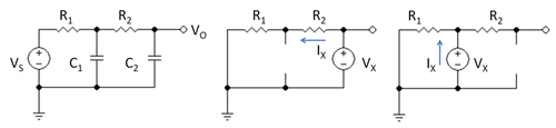
Figure 1 shows a simple RC low-pass filter. Its transfer functionTransfer function
A transfer function is a mathematical representation, in terms of spatial or temporal frequency, of the relation between the input and output of a linear time-invariant system. With optical imaging devices, for example, it is the Fourier transform of the point spread function i.e...
is found using Kirchhoff's current law
Kirchhoff's laws
There are several Kirchhoff's laws, all named after Gustav Robert Kirchhoff:* Kirchhoff's circuit laws* Kirchhoff's law of thermal radiation* Kirchhoff's equations* Kirchhoff's three laws of spectroscopy* Kirchhoff's law of thermochemistry-See also:...
as follows. At the output,
where V1 is the voltage at the top of capacitor C1. At the center node:
Combining these relations the transfer function is found to be:
The linear term in jω in this transfer function can be derived by the following method, which is an application of the open-circuit time constant method to this example.
- Set the signal source to zero.
- Select capacitor C2, replace it by a test voltage VX, and replace C1 by an open circuit. Then the resistance seen by the test voltage is found using the circuit in the middle panel of Figure 1 and is simply VX / IX = R1 + R2. Form the product C2 ( R1 + R2 ).
- Select capacitor C1, replace it by a test voltage VX, and replace C2 by an open circuit. Then the resistance seen by the test voltage is found using the circuit in the right panel of Figure 1 and is simply VX / IX = R1. Form the product C1 R1.
- Add these terms.
In effect, it is as though each capacitor charges and discharges through the resistance found in the circuit when the other capacitor is an open circuit.
The open circuit time constant procedure provides the linear term in jω regardless of how complex the RC network becomes. For a complex circuit, the procedure consists of following the above rules, going through all the capacitors in the circuit. A more general derivation is found in Gray and Meyer.
So far the result is general, but an approximation is introduced to make use of this result: the assumption is made that this linear term in jω determines the corner frequency of the circuit.
That assumption can be examined more closely using the example of Figure 1: suppose the time constants of this circuit are τ1 and τ2; that is:

Comparing the coefficients of the linear and quadratic terms in jω, there results:

One of the two time constants will be the longest; let it be τ1. Suppose for the moment that it is much larger than the other, τ1 >> τ2. In this case, the approximations hold that:

and
In other words, substituting the RC-values:

and
where ( ^ ) denotes the approximate result. As an aside, notice that the circuit time constants both involve both capacitors; in other words, in general the circuit time constants are not decided by any single capacitor. Using these results, it is easy to explore how well the corner frequency (the 3dB frequency) is given by

-
 with
with 
Of course agreement is good when the assumption τ1 >> τ2 is accurate.
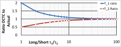
Figure 2 illustrates the approximation. The x-axis is the ratio τ1 / τ2 on a logarithmic scale. An increase in this variable means the higher pole is further above the corner frequency. The y-axis is the ratio of the OCTC (open-circuit time constant) estimate to the true time constant. For the lowest pole use curve T_1; this curve refers to the corner frequency; and for the higher pole use curve T_2. The worst agreement is for τ1 = τ2. In this case τ^1 = 2 τ1 and the corner frequency is a factor of 2 too small. The higher pole is a factor of 2 too high (its time constant is half of the real value).
In all cases, the estimated corner frequency is closer than a factor of two from the real one, and always is conservative that is, lower than the real corner, so the actual circuit will behave better than predicted. However, the higher pole always is optimistic, that is, predicts the high pole at a higher frequency than really is the case. To use these estimates for step response predictions, which depend upon the ratio of the two pole frequencies (see article on pole splitting for an example), Figure 2 suggests a fairly large ratio of τ1 / τ2 is needed for accuracy because the errors in τ^1 and τ^2 reinforce each other in the ratio τ^1 / τ^2.
The open-circuit time constant method focuses upon the corner frequency alone, but as seen above, estimates for higher poles also are possible.
Application of the open-circuit time constant method to a number of single transistor amplifier stages can be found in Pittet and Kandaswamy.