
Ice-type model
Encyclopedia
In statistical mechanics
, the ice-type models or six-vertex models are a family of vertex model
s for crystal lattices with hydrogen bonds. The first such model was introduced by Linus Pauling
in 1935 to account for the residual entropy
of water ice. Variants have been proposed as models of certain ferroelectric and antiferroelectric crystals.
In 1967, Elliott H. Lieb
found the exact solution to a two-dimensional ice model known as "square ice". The exact solution in three dimensions is only known for a special "frozen" state.
4 - that is, each vertex of the lattice is connected by an edge to four "nearest neighbours". A state of the model consists of an arrow on each edge of the lattice, such that the number of arrows pointing inwards at each vertex is 2. This restriction on the arrow configurations is known as the ice rule.
For two-dimensional models, the lattice is taken to be the square lattice. For more realistic models, one can use a three-dimensional lattice appropriate to the material being considered; for example, the hexagonal ice lattice
is used to analyse ice.
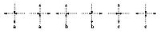
At any vertex, there are six configurations of the arrows which satisfy the ice rule (justifying the name "six-vertex model"). The valid configurations for the (two-dimensional) square lattice are the following:
The energy of a state is understood to be a function of the configurations at each vertex. For square lattices, one assumes that the total energy is given by

for some constants , where
  here denotes the number of vertices with the
  th configuration from the above figure. The value
  is the energy associated with vertex configuration number
  .
.
One aims to calculate the partition function
 of an ice-type model, which is given by the formula
where the sum is taken over all states of the model, and where is the energy of the state,
  is Boltzmann's constant, and
  is the system's temperature.
Typically, one is interested in the thermodynamic limit
in which the number of vertices approaches infinity. In that case, one instead evaluates the free energy per vertex
  in the limit as
  , where
  is given by
Equivalently, one evaluates the partition function per vertex in the thermodynamic limit, where

The values and
and  are related by
In ice, each oxygen atom is connected by a bond to four other oxygens, and each bond contains one hydrogen atom between the terminal oxygens. The hydrogen occupies one of two symmetrically located positions, neither of which is in the middle of the bond. Pauling argued that the allowed configuration of hydrogen atoms is such that there are always exactly two hydrogens close to each oxygen, thus making the local environment imitate that of a water molecule, . Thus, if we take the oxygen atoms as the lattice vertices and the hydrogen bonds as the lattice edges, and if we draw an arrow on a bond which points to the side of the bond on which the hydrogen atom sits, then ice satisfies the ice model.
Similar reasoning applies to show that KDP also satisfies the ice model.
 associated with vertex configurations 1-6 determine the relative probabilities of states, and thus can influence the macroscopic behaviour of the system. The following are common choices for these vertex energies.
 , as all permissible vertex configurations are understood to be equally likely. In this case, the partition function
  equals the total number of valid states. This model is known as the ice model (as opposed to an ice-type model).

For this model (called the KDP model), the most likely state (the least-energy state) has all horizontal arrows pointing in the same direction, and likewise for all vertical arrows. Such a state is a ferroelectric state, in which all hydrogen atoms have a preference for one fixed side of their bonds.
Rys
The Rys  model is obtained by setting

The least-energy state for this model is dominated by vertex configurations 5 and 6. For such a state, adjacent horizontal bonds necessarily have arrows in opposite directions and similarly for vertical bonds, so this state is an antiferroelectric state.

This assumption is known as the zero field assumption, and holds for the ice model, the KDP model, and the Rys F model.
of ice that had been measured by William F. Giauque and E. L. Stout. The residual entropy, , of ice is given by the formula

where is Boltzmann's constant,
  is the number of oxygen atoms in the piece of ice, which is always taken to be large (the thermodynamic limit
) and is the number of configurations of the hydrogen atoms according to Pauling's ice rule. Without the ice rule we would have
  since the number of hydrogen atoms is
  and each hydrogen has two possible locations. Pauling estimated that the ice rule reduces this to
  , a number that would agree extremely well with the Giauque-Stout measurement of
  . It can be said that Pauling's calculation of
  for ice is one of the simplest, yet most accurate applications of statistical mechanics
to real substances ever made. The question that remained was whether, given the model, Pauling's calculation of , which was very approximate, would be sustained by a rigorous calculation. This became a significant problem in combinatorics
.
Both the three-dimensional and two-dimensional models were computed numerically by John F. Nagle in 1966 who found that in three-dimensions and
  in two-dimensions. Both are amazingly close to Pauling's rough calculation, 1.5.
In 1967, Lieb found the exact solution of three two-dimensional ice-type models: the ice model, the Rys model, and the KDP model. The solution for the ice model gave the exact value of
  in two-dimensions as
which is known as Lieb's square ice constant
.
Later in 1967, Bill Sutherland generalised Lieb's solution of the three specific ice-type models to a general exact solution for square-lattice ice-type models satisfying the zero field assumption.
Still later in 1967, C. P. Yang generalised Sutherland's solution to an exact solution for square-lattice ice-type models in a horizontal electric field.
In 1969, John Nagle derived the exact solution for a three-dimensional version of the KDP model, for a specific range of temperatures. For such temperatures, the model is "frozen" in the sense that (in the thermodynamic limit) the energy per vertex and entropy per vertex are both zero. This is the only known exact solution for a three-dimensional ice-type model.
, which has also been exactly solved, is a generalisation of the (square-lattice) six-vertex model: to recover the six-vertex model from the eight-vertex model, set the energies for vertex configurations 7 and 8 to infinity. Six-vertex models have been solved in some cases for which the eight-vertex model has not; for example, Nagle's solution for the three-dimensional KDP model and Yang's solution of the six-vertex model in a horizontal field.
the bulk free energy in the thermodynamic limit
depends on boundary conditions. The model was analytically solved for periodic boundary conditions, anti-periodic,
ferromagnetic and domain wall boundary conditions. Six vertex model with domain wall boundary conditions on a square lattice has specific significance for algebraic combinatorics, it helps to enumerate Alternating sign matrix
.
In this case the partition function can be represented as a determinant of a matrix (dimension of the matrix is equal to the size of the lattice), but in the other cases the enumeration of
 does not come out in such a simple closed form.
Domain wall gives the smallest . Clearly, the largest
is given by free boundary conditions (no constraint at all on the configurations on the boundary), but the same occurs, in the thermodynamic limit, for periodic boundary conditions, as used originally to derive
  .
.
on the edge to an adjacent square goes left or right (according to an observer in the square) depending on whether the color in the adjacent square is i+1 or i−1 mod 3. There are 3 possible ways to color a fixed initial square, and once this initial color is chosen this gives a 1:1 correspondence between colorings and arrangements of arrows satisfying the ice-type condition.
Statistical mechanics
Statistical mechanics or statistical thermodynamicsThe terms statistical mechanics and statistical thermodynamics are used interchangeably...
, the ice-type models or six-vertex models are a family of vertex model
Vertex model
A vertex model is a type of statistical mechanics model in which the Boltzmann weights are associated with a vertex in the model . This contrasts with a nearest-neighbour model, such as the Ising model, in which the energy, and thus the Boltzmann weight of a statistical microstate is attributed to...
s for crystal lattices with hydrogen bonds. The first such model was introduced by Linus Pauling
Linus Pauling
Linus Carl Pauling was an American chemist, biochemist, peace activist, author, and educator. He was one of the most influential chemists in history and ranks among the most important scientists of the 20th century...
in 1935 to account for the residual entropy
Residual entropy
Residual entropy is small amount of entropy which is present even after a substance is cooled arbitrarily close to absolute zero. It occurs if a material can exist in many different microscopic states when cooled to absolute zero...
of water ice. Variants have been proposed as models of certain ferroelectric and antiferroelectric crystals.
In 1967, Elliott H. Lieb
Elliott H. Lieb
Elliott H. Lieb is an eminent American mathematical physicist and professor of mathematics and physics at Princeton University who specializes in statistical mechanics, condensed matter theory, and functional analysis....
found the exact solution to a two-dimensional ice model known as "square ice". The exact solution in three dimensions is only known for a special "frozen" state.
Description
An ice-type model is a lattice model defined on a lattice of coordination numberCoordination number
In chemistry and crystallography, the coordination number of a central atom in a molecule or crystal is the number of its nearest neighbours. This number is determined somewhat differently for molecules and for crystals....
4 - that is, each vertex of the lattice is connected by an edge to four "nearest neighbours". A state of the model consists of an arrow on each edge of the lattice, such that the number of arrows pointing inwards at each vertex is 2. This restriction on the arrow configurations is known as the ice rule.
For two-dimensional models, the lattice is taken to be the square lattice. For more realistic models, one can use a three-dimensional lattice appropriate to the material being considered; for example, the hexagonal ice lattice
Ice Ih
thumb|Photograph showing details of an ice cube under magnification. Ice Ih is the form of ice commonly seen on earth.Ice Ih is the hexagonal crystal form of ordinary ice, or frozen water. Virtually all ice in the biosphere is ice Ih, with the exception only of a small amount of ice Ic which is...
is used to analyse ice.
At any vertex, there are six configurations of the arrows which satisfy the ice rule (justifying the name "six-vertex model"). The valid configurations for the (two-dimensional) square lattice are the following:
The energy of a state is understood to be a function of the configurations at each vertex. For square lattices, one assumes that the total energy
is given byfor some constants
, where here denotes the number of vertices with the th configuration from the above figure. The value is the energy associated with vertex configuration number .One aims to calculate the partition function
Partition function (statistical mechanics)
Partition functions describe the statistical properties of a system in thermodynamic equilibrium. It is a function of temperature and other parameters, such as the volume enclosing a gas...
of an ice-type model, which is given by the formulawhere the sum is taken over all states of the model, and where
is the energy of the state, is Boltzmann's constant, and is the system's temperature.Typically, one is interested in the thermodynamic limit
Thermodynamic limit
In thermodynamics, particularly statistical mechanics, the thermodynamic limit is reached as the number of particles in a system, N, approaches infinity...
in which the number
of vertices approaches infinity. In that case, one instead evaluates the free energy per vertex in the limit as , where is given byEquivalently, one evaluates the partition function per vertex
in the thermodynamic limit, whereThe values
and are related byPhysical justification
Several real crystals with hydrogen bonds satisfy the ice model, including ice and potassium dihydrogen phosphate (KDP). Indeed, such crystals motivated the study of ice-type models.In ice, each oxygen atom is connected by a bond to four other oxygens, and each bond contains one hydrogen atom between the terminal oxygens. The hydrogen occupies one of two symmetrically located positions, neither of which is in the middle of the bond. Pauling argued that the allowed configuration of hydrogen atoms is such that there are always exactly two hydrogens close to each oxygen, thus making the local environment imitate that of a water molecule, . Thus, if we take the oxygen atoms as the lattice vertices and the hydrogen bonds as the lattice edges, and if we draw an arrow on a bond which points to the side of the bond on which the hydrogen atom sits, then ice satisfies the ice model.
Similar reasoning applies to show that KDP also satisfies the ice model.
Specific choices of vertex energies
On the square lattice, the energies associated with vertex configurations 1-6 determine the relative probabilities of states, and thus can influence the macroscopic behaviour of the system. The following are common choices for these vertex energies.The ice model
When modelling ice, one takes, as all permissible vertex configurations are understood to be equally likely. In this case, the partition function equals the total number of valid states. This model is known as the ice model (as opposed to an ice-type model).The KDP model of a ferroelectric
Slater argued that KDP could be represented by an ice-type model with energiesFor this model (called the KDP model), the most likely state (the least-energy state) has all horizontal arrows pointing in the same direction, and likewise for all vertical arrows. Such a state is a ferroelectric state, in which all hydrogen atoms have a preference for one fixed side of their bonds.
Rys  model of an antiferroelectric
The Rys model is obtained by settingThe least-energy state for this model is dominated by vertex configurations 5 and 6. For such a state, adjacent horizontal bonds necessarily have arrows in opposite directions and similarly for vertical bonds, so this state is an antiferroelectric state.
The zero field assumption
If there is no ambient electric field, then the total energy of a state should remain unchanged under a charge reversal, i.e. under flipping all arrows. Thus one may assume without loss of generality thatThis assumption is known as the zero field assumption, and holds for the ice model, the KDP model, and the Rys F model.
History
The ice rule was introduced by Linus Pauling in 1935 to account for the residual entropyResidual entropy
Residual entropy is small amount of entropy which is present even after a substance is cooled arbitrarily close to absolute zero. It occurs if a material can exist in many different microscopic states when cooled to absolute zero...
of ice that had been measured by William F. Giauque and E. L. Stout. The residual entropy,
, of ice is given by the formulawhere
is Boltzmann's constant, is the number of oxygen atoms in the piece of ice, which is always taken to be large (the thermodynamic limitThermodynamic limit
In thermodynamics, particularly statistical mechanics, the thermodynamic limit is reached as the number of particles in a system, N, approaches infinity...
) and
is the number of configurations of the hydrogen atoms according to Pauling's ice rule. Without the ice rule we would have since the number of hydrogen atoms is and each hydrogen has two possible locations. Pauling estimated that the ice rule reduces this to , a number that would agree extremely well with the Giauque-Stout measurement of . It can be said that Pauling's calculation of for ice is one of the simplest, yet most accurate applications of statistical mechanicsStatistical mechanics
Statistical mechanics or statistical thermodynamicsThe terms statistical mechanics and statistical thermodynamics are used interchangeably...
to real substances ever made. The question that remained was whether, given the model, Pauling's calculation of
, which was very approximate, would be sustained by a rigorous calculation. This became a significant problem in combinatoricsCombinatorics
Combinatorics is a branch of mathematics concerning the study of finite or countable discrete structures. Aspects of combinatorics include counting the structures of a given kind and size , deciding when certain criteria can be met, and constructing and analyzing objects meeting the criteria ,...
.
Both the three-dimensional and two-dimensional models were computed numerically by John F. Nagle in 1966 who found that
in three-dimensions and in two-dimensions. Both are amazingly close to Pauling's rough calculation, 1.5.In 1967, Lieb found the exact solution of three two-dimensional ice-type models: the ice model, the Rys
model, and the KDP model. The solution for the ice model gave the exact value of in two-dimensions aswhich is known as Lieb's square ice constant
Lieb's square ice constant
Lieb's square ice constant is a mathematical constant used in the field of combinatorics. It was introduced by Elliott H. Lieb in 1967.-Definition:...
.
Later in 1967, Bill Sutherland generalised Lieb's solution of the three specific ice-type models to a general exact solution for square-lattice ice-type models satisfying the zero field assumption.
Still later in 1967, C. P. Yang generalised Sutherland's solution to an exact solution for square-lattice ice-type models in a horizontal electric field.
In 1969, John Nagle derived the exact solution for a three-dimensional version of the KDP model, for a specific range of temperatures. For such temperatures, the model is "frozen" in the sense that (in the thermodynamic limit) the energy per vertex and entropy per vertex are both zero. This is the only known exact solution for a three-dimensional ice-type model.
Relation to eight-vertex model
The eight-vertex modelEight-vertex model
In statistical mechanics, the eight-vertex model is a generalisation of the ice-type models; it was discussed by Sutherland, and Fan & Wu, and solved by Baxter in the zero-field case.-Description:...
, which has also been exactly solved, is a generalisation of the (square-lattice) six-vertex model: to recover the six-vertex model from the eight-vertex model, set the energies for vertex configurations 7 and 8 to infinity. Six-vertex models have been solved in some cases for which the eight-vertex model has not; for example, Nagle's solution for the three-dimensional KDP model and Yang's solution of the six-vertex model in a horizontal field.
Boundary conditions
This ice model provide an important 'counterexample' in statistical mechanics:the bulk free energy in the thermodynamic limit
Thermodynamic limit
In thermodynamics, particularly statistical mechanics, the thermodynamic limit is reached as the number of particles in a system, N, approaches infinity...
depends on boundary conditions. The model was analytically solved for periodic boundary conditions, anti-periodic,
ferromagnetic and domain wall boundary conditions. Six vertex model with domain wall boundary conditions on a square lattice has specific significance for algebraic combinatorics, it helps to enumerate Alternating sign matrix
Alternating sign matrix
In mathematics, an alternating sign matrix is a square matrix of 0s, 1s, and −1s such that the sum of each row and column is 1 and the nonzero entries in each row and column alternate in sign. These matrices arise naturally when using Dodgson condensation to compute a determinant...
.
In this case the partition function can be represented as a determinant of a matrix (dimension of the matrix is equal to the size of the lattice), but in the other cases the enumeration of
does not come out in such a simple closed form.Domain wall gives the smallest
. Clearly, the largestis given by free boundary conditions (no constraint at all on the configurations on the boundary), but the same
occurs, in the thermodynamic limit, for periodic boundary conditions, as used originally to derive .3-colorings of a lattice
The number of states of an ice type model on the internal edges of a finite simply connected union of squares of a lattice is equal to one third of the number of ways to 3-color the squares, with no two adjacent squares having the same color. This correspondence between states is due to Andrew Lenard and is given as follows. If a square has color i = 0, 1, or 2, then the arrowon the edge to an adjacent square goes left or right (according to an observer in the square) depending on whether the color in the adjacent square is i+1 or i−1 mod 3. There are 3 possible ways to color a fixed initial square, and once this initial color is chosen this gives a 1:1 correspondence between colorings and arrangements of arrows satisfying the ice-type condition.