

Elliptic curve point multiplication
Encyclopedia
Elliptic curve point multiplication is the operation of successively adding a point along an elliptic curve
to itself repeatedly. It is used in elliptic curve cryptography
as a means of producing a trap door function.
 ) we define point multiplication as the repeated addition of a point along that curve. Denote as
  for some scalar (integer) n and a point
  that lies on the curve E.
The security of modern ECC depends on the intractability of determining n from given known values of Q and P. It is known as the elliptic curve discrete logarithm problem.
Compute dP with the following representation
* Q = 0
* for i from m to 0 do
* Q := 2Q (using point doubling)
* if di = 1 then Q := Q + P (using point addition)
* Return Q
An alternative way of writing the above as a recursive function is
where f is the function for doubling, P is the coordinate to double, n is the number of times to double the coordinate. Example: 100P can be written as 2(2(P+2(2(2(P+2P))))) and thus requires six doublings and two additions. 100P would be equal to f(P,100).
This algorithm requires iterations of point doubling and addition to compute the full point multiplication. There are many variations of this algorithm such as using a window, sliding window, NAF, NAF-w, vector chains, and Montgomery Ladder.
 values of
  for
for  . The algorithm now uses the representation
  and becomes
* Q = 0
* for i from 0 to m do
* Q := 2wQ (using repeated point doubling)
* if di > 0 then Q := Q + diP (using a single point addition with the pre-computed value of diP)
* Return Q
This algorithm has the same complexity as the double-and-add approach with the benefit of using fewer point additions (which in practice are slower than doubling). Typically, the value of w is chosen to be fairly small making the pre-computation stage a trivial component of the algorithm. For the NIST recommended curves is usually the best selection. The entire complexity for a n-bit number is measured as
  point doubles and
  point additions.
 for
for  . Effectively, we are only computing the values for which the most significant bit of the window is set. The algorithm then uses the original double-and-add representation of
  .
.
* Q = 0
* for i from 0 to m do
* if di = 0 then
* Q := 2Q (point double)
* else
* Grab up to w - 1 additional bits from d to store into (including di) t and decrement i suitably
* If fewer than w bits were grabbed
* Perform double-and-add using t
* Return Q
* else
* Q := 2wQ (repeated point double)
* Q := Q + tP (point addition)
* Return Q
This algorithm has the benefit that the pre-computation stage is roughly half as complex as the normal windowed method while also trading slower point additions for point doublings. In effect, there is little reason to use the windowed method over this approach. The algorithm requires point doubles and at most
  point additions.
we aim to make use of the fact that point subtraction is just as easy as point addition to perform fewer (of either) as compared to a sliding-window method. The NAF of the multiplicand must be computed first with the following algorithm
* i = 0
* While (d > 0) do
* if (d mod 2) 1 then
* di = d mods 2w
* d = d - di
* else
* di = 0
* d = d/2
* i = i + 1
* return (di-1, di-2, ..., d0)
Where the mods function is defined as
* if d >= 2w-1
* return (d mod 2w) - 2w
* else
* return d mod 2w
This produces the NAF we need to now perform the multiplication. This algorithm requires the pre-computation of the points and their negatives. On typical Weierstrass curves if
  then
then  . So in essence the negatives are cheap to compute. Next, the following algorithm computes the multiplication
  :
:
* Q = 0
* for j = i-1 downto 0 do
* Q = 2Q
* if (dj != 0)
* Q = Q + djP
* return Q
The wNAF guarantees that on average there will be a density of point additions (slightly better than the unsigned window). It requires 1 point doubling and
  point additions for precomputation. The algorithm then requires
  point doublings and
  point additions for the rest of the multiplication.
One property of the NAF is that we are guaranteed that every non-zero element is followed by at least
  additional zeroes. This is because the algorithm clears out the lower
  bits of
  with every subtraction of the output of the mods function. This observation can be used for several purposes. After every non-zero element the additional zeroes can be implied and do not need to be stored. Secondly, the multiple serial divisions by 2 can be replaced by a division by
  after every non-zero
  element and divide by 2 after every zero.
Montgomery ladder
The Montgomery ladder approach computes the point multiplication in a fixed amount of time. This can be beneficial when timing or power consumption measurements are exposed to an attacker performing a side channel attack. The algorithm uses the same representation as from double-and-add.
* R0 := 0
* R1 := P
* for i from m to 0 do
* if di = 0 then
* R1 := R0 + R1
* R0 := 2R0
* else
* R0 := R0 + R1
* R1 := 2R1
* Return R0
This algorithm is in effect the same speed as the double-and-add approach except that it computes the same number of point additions and doubles regardless of the value of the multiplicand d. This means that at this level the algorithm does not leak any information through timing or power.
Elliptic curve
In mathematics, an elliptic curve is a smooth, projective algebraic curve of genus one, on which there is a specified point O. An elliptic curve is in fact an abelian variety — that is, it has a multiplication defined algebraically with respect to which it is a group — and O serves as the identity...
to itself repeatedly. It is used in elliptic curve cryptography
Elliptic curve cryptography
Elliptic curve cryptography is an approach to public-key cryptography based on the algebraic structure of elliptic curves over finite fields. The use of elliptic curves in cryptography was suggested independently by Neal Koblitz and Victor S...
as a means of producing a trap door function.
Basics
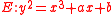
Given a curve E defined along some equation in a finite field (such as) we define point multiplication as the repeated addition of a point along that curve. Denote as for some scalar (integer) n and a point that lies on the curve E.The security of modern ECC depends on the intractability of determining n from
given known values of Q and P. It is known as the elliptic curve discrete logarithm problem.Point addition
Point addition is defined as taking two points along a curve E and computing where a line through them intersects the curve. We use the negative of the intersection point as the result of the addition.Point doubling
Like point addition except we take the tangent of a single point and find the intersection with the tangent line.Point multiplication
The straight forward way of computing a point multiplication is through repeated addition (with the exception of the first addition since adding a point to itself is usually undefined since the slope of the line through the point is 0). However, this is a fully exponential approach to computing the multiplication.Double-and-add
The simplest method is the double-and-add method similar to multiply-and-square in modular exponentiation. The algorithm works as follows:Compute dP with the following representation
* Q = 0
* for i from m to 0 do
* Q := 2Q (using point doubling)
* if di = 1 then Q := Q + P (using point addition)
* Return Q
An alternative way of writing the above as a recursive function is
f(P, n) is

   if n = 0 then return 0           # computation complete

   else if n mod 2 = 1 then

      P + f(P, n-1)                 # addition when n is odd

   else

      f(2P, n/2)                    # doubling when n is even
where f is the function for doubling, P is the coordinate to double, n is the number of times to double the coordinate. Example: 100P can be written as 2(2(P+2(2(2(P+2P))))) and thus requires six doublings and two additions. 100P would be equal to f(P,100).
This algorithm requires
iterations of point doubling and addition to compute the full point multiplication. There are many variations of this algorithm such as using a window, sliding window, NAF, NAF-w, vector chains, and Montgomery Ladder.Windowed method
In the windowed version of this algorithm we select a window size w and compute all values of for . The algorithm now uses the representation and becomes* Q = 0
* for i from 0 to m do
* Q := 2wQ (using repeated point doubling)
* if di > 0 then Q := Q + diP (using a single point addition with the pre-computed value of diP)
* Return Q
This algorithm has the same complexity as the double-and-add approach with the benefit of using fewer point additions (which in practice are slower than doubling). Typically, the value of w is chosen to be fairly small making the pre-computation stage a trivial component of the algorithm. For the NIST recommended curves
is usually the best selection. The entire complexity for a n-bit number is measured as point doubles and point additions.Sliding-window method
In the sliding-window version we look to trade off point additions for point doubles. We compute a similar table as in the windowed version except we only compute the points for . Effectively, we are only computing the values for which the most significant bit of the window is set. The algorithm then uses the original double-and-add representation of .* Q = 0
* for i from 0 to m do
* if di = 0 then
* Q := 2Q (point double)
* else
* Grab up to w - 1 additional bits from d to store into (including di) t and decrement i suitably
* If fewer than w bits were grabbed
* Perform double-and-add using t
* Return Q
* else
* Q := 2wQ (repeated point double)
* Q := Q + tP (point addition)
* Return Q
This algorithm has the benefit that the pre-computation stage is roughly half as complex as the normal windowed method while also trading slower point additions for point doublings. In effect, there is little reason to use the windowed method over this approach. The algorithm requires
point doubles and at most point additions.wNAF Method
In the Non-Adjacent FormNon-adjacent form
The non-adjacent form of a number is a unique signed-digit representation. Like the name suggests, non-zero values cannot be adjacent. For example:2 = 4 + 2 + 1 = 72 = 8 − 2 + 1 = 72 = 8 − 4 + 2 + 1 = 72 = 8 − 1 = 7...
we aim to make use of the fact that point subtraction is just as easy as point addition to perform fewer (of either) as compared to a sliding-window method. The NAF of the multiplicand
must be computed first with the following algorithm* i = 0
* While (d > 0) do
* if (d mod 2) 1 then
* di = d mods 2w
* d = d - di
* else
* di = 0
* d = d/2
* i = i + 1
* return (di-1, di-2, ..., d0)
Where the mods function is defined as
* if d >= 2w-1
* return (d mod 2w) - 2w
* else
* return d mod 2w
This produces the NAF we need to now perform the multiplication. This algorithm requires the pre-computation of the points
and their negatives. On typical Weierstrass curves if then . So in essence the negatives are cheap to compute. Next, the following algorithm computes the multiplication :* Q = 0
* for j = i-1 downto 0 do
* Q = 2Q
* if (dj != 0)
* Q = Q + djP
* return Q
The wNAF guarantees that on average there will be a density of
point additions (slightly better than the unsigned window). It requires 1 point doubling and point additions for precomputation. The algorithm then requires point doublings and point additions for the rest of the multiplication.One property of the NAF is that we are guaranteed that every non-zero element
is followed by at least additional zeroes. This is because the algorithm clears out the lower bits of with every subtraction of the output of the mods function. This observation can be used for several purposes. After every non-zero element the additional zeroes can be implied and do not need to be stored. Secondly, the multiple serial divisions by 2 can be replaced by a division by after every non-zero element and divide by 2 after every zero.Montgomery ladder
The Montgomery ladder approach computes the point multiplication in a fixed amount of time. This can be beneficial when timing or power consumption measurements are exposed to an attacker performing a side channel attack. The algorithm uses the same representation as from double-and-add.
* R0 := 0
* R1 := P
* for i from m to 0 do
* if di = 0 then
* R1 := R0 + R1
* R0 := 2R0
* else
* R0 := R0 + R1
* R1 := 2R1
* Return R0
This algorithm is in effect the same speed as the double-and-add approach except that it computes the same number of point additions and doubles regardless of the value of the multiplicand d. This means that at this level the algorithm does not leak any information through timing or power.