Derivation of the Routh array
Encyclopedia
The Routh array is a tabular method permitting one to establish the stability
of a system using only the coefficients of the characteristic polynomial
. Central to the field of control systems design
, the Routh–Hurwitz theorem
and Routh array emerge by using the Euclidean algorithm
and Sturm's theorem
in evaluating Cauchy indices
.
Stable polynomial
A polynomial is said to be stable if either:* all its roots lie in the open left half-plane, or* all its roots lie in the open unit disk.The first condition defines Hurwitz stability and the second one Schur stability. Stable polynomials arise in various mathematical fields, for example in...
of a system using only the coefficients of the characteristic polynomial
Polynomial
In mathematics, a polynomial is an expression of finite length constructed from variables and constants, using only the operations of addition, subtraction, multiplication, and non-negative integer exponents...
. Central to the field of control systems design
Control theory
Control theory is an interdisciplinary branch of engineering and mathematics that deals with the behavior of dynamical systems. The desired output of a system is called the reference...
, the Routh–Hurwitz theorem
Routh–Hurwitz theorem
In mathematics, Routh–Hurwitz theorem gives a test to determine whether a given polynomial is Hurwitz-stable. It was proved in 1895 and named after Edward John Routh and Adolf Hurwitz.-Notations:...
and Routh array emerge by using the Euclidean algorithm
Euclidean algorithm
In mathematics, the Euclidean algorithm is an efficient method for computing the greatest common divisor of two integers, also known as the greatest common factor or highest common factor...
and Sturm's theorem
Sturm's theorem
In mathematics, Sturm's theorem is a symbolic procedure to determine the number of distinct real roots of a polynomial. It was named for Jacques Charles François Sturm...
in evaluating Cauchy indices
Cauchy index
In mathematical analysis, the Cauchy index is an integer associated to a real rational function over an interval. By the Routh-Hurwitz theorem, we have the following interpretation: the Cauchy index of...
.
The Cauchy index
Given the system:-

Assuming no roots of lie on the imaginary axis, and letting
-
 = The number of roots of
  with negative real parts, and
 -
 = The number of roots of
  with positive real parts
then we have
Expressing in polar form, we have
where
and
from (2) note that
where
Now if the ith root of has a positive real part, then (using the notation y=(RE[y],IM[y]))
-
and
Similarly, if the ith root of has a negative real part,
and
Therefore,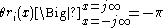 when the ith root of
  has a positive real part, and
  when the ith root of
  has a negative real part. Alternatively,
and
So, if we define
then we have the relationship

and combining (3) and (16) gives us
-
 and
and 
Therefore, given an equation of of degree
  we need only evaluate this function
  to determine
  , the number of roots with negative real parts and
  , the number of roots with positive real parts.
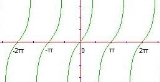
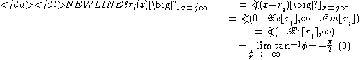
.jpg)
Figure 1  versus
Equations (13) and (14) show that at ,
,  is an integer multiple of
  . Note now, in accordance with (6) and Figure 1, the graph of
  vs
vs  , that varying
  over an interval (a,b) where
  and
and  are integer multiples of
  , this variation causing the function
  to have increased by
  , indicates that in the course of travelling from point a to point b,
  has "jumped" from
  to
to  one more time than it has jumped from
  to
to  . Similarly, if we vary
  over an interval (a,b) this variation causing
  to have decreased by
  , where again
  is a multiple of
  at both
  and
and  , implies that
  has jumped from
  to
to  one more time than it has jumped from
  to
to  as
as  was varied over the said interval.
Thus, is
is  times the difference between the number of points at which
  jumps from
  to
to  and the number of points at which
 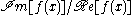 jumps from
  to
to  as
as  ranges over the interval
  provided that at
  ,
,  is defined.
.svg.png)
Figure 2  versus
In the case where the starting point is on an incongruity (i.e. , i = 0, 1, 2, ...) the ending point will be on an incongruity as well, by equation (16) (since
  is an integer and
  is an integer,
  will be an integer). In this case, we can achieve this same index (difference in positive and negative jumps) by shifting the axes of the tangent function by
  , through adding
  to
to  . Thus, our index is now fully defined for any combination of coefficients in
  by evaluating
  over the interval (a,b) =
  when our starting (and thus ending) point is not an incongruity, and by evaluating
over said interval when our starting point is at an incongruity.
This difference, , of negative and positive jumping incongruities encountered while traversing
  from
from  to
to  is called the Cauchy Index of the tangent of the phase angle, the phase angle being
  or
or  , depending as
  is an integer multiple of
  or not.
The Routh criterion
To derive Routh's criterion, first we'll use a different notation to differentiate between the even and odd terms of :
:
Now we have:
-

Therefore, if is even,
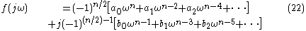
and if is odd:
-

Now observe that if is an odd integer, then by (3)
  is odd. If
  is an odd integer, then
  is odd as well. Similarly, this same argument shows that when
  is even,
  will be even. Equation (13) shows that if
  is even,
  is an integer multiple of
  . Therefore,
  is defined for
  even, and is thus the proper index to use when n is even, and similarly
  is defined for
  odd, making it the proper index in this latter case.
Thus, from (6) and (22), for even:
even:
and from (18) and (23), for odd:
odd:

Lo and behold we are evaluating the same Cauchy index for both:
Sturm's theorem
Sturm gives us a method for evaluating . His theorem states as follows:
Given a sequence of polynomials where:
1) If then
then  ,
,  , and
, and 
2) for
for 
and we define as the number of changes of sign in the sequence
  for a fixed value of
  , then:
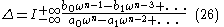
A sequence satisfying these requirements is obtained using the Euclidean algorithm, which is as follows:
Starting with and
and  , and denoting the remainder of
  by
by  and similarly denoting the remainder of
  by
by  , and so on, we obtain the relationships:
or in general
where the last non-zero remainder, will therefore be the highest common factor of
  . It can be observed that the sequence so constructed will satisfy the conditions of Sturm's theorem, and thus an algorithm for determining the stated index has been developed.
It is in applying Sturm's theorem (28) to (26), through the use of the Euclidean algorithm above that the Routh matrix is formed.
We get
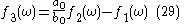
and identifying the coefficients of this remainder by ,
,  ,
,  ,
,  , and so forth, makes our formed remainder

where

Continuing with the Euclidean algorithm on these new coefficients gives us
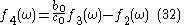
where we again denote the coefficients of the remainder by
by  ,
,  ,
,  ,
,  ,
,
making our formed remainder

and giving us

The rows of the Routh array are determined exactly by this algorithm when applied to the coefficients of (19). An observation worthy of note is that in the regular case the polynomials and
and  have as the highest common factor
  and thus there will be
  polynomials in the chain
  .
.
Note now, that in determining the signs of the members of the sequence of polynomials that at
  the dominating power of
  will be the first term of each of these polynomials, and thus only these coefficients corresponding to the highest powers of
  in
in  , and
, and  , which are
  ,
,  ,
,  ,
,  , ... determine the signs of
  ,
,  , ...,
  at
at  .
.
So we get that is,
  is the number of changes of sign in the sequence
  ,
,  ,
,  , ... which is the number of sign changes in the sequence
  ,
,  ,
,  ,
,  , ... and
  ; that is
  is the number of changes of sign in the sequence
  ,
,  ,
,  , ... which is the number of sign changes in the sequence
  ,
,  ,
,  ,
,  , ...
, ...
Since our chain ,
,  ,
,  ,
,  , ... will have
  members it is clear that
  since within
 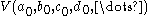 if going from
  to
to  a sign change has not occurred, within
 going from
  to
to  one has, and likewise for all
  transitions (there will be no terms equal to zero) giving us
  total sign changes.
As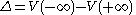 and
and  , and from (17)
  , we have that
  and have derived Routh's theorem -
The number of roots of a real polynomial which lie in the right half plane
  is equal to the number of changes of sign in the first column of the Routh scheme.
And for the stable case where then
then  by which we have Routh's famous criterion:
In order for all the roots of the polynomial to have negative real parts, it is necessary and sufficient that all of the elements in the first column of the Routh scheme be different from zero and of the same sign.
-
-
-
-