

Brent's method
Encyclopedia
In numerical analysis
, Brent's method is a complicated but popular root-finding algorithm
combining the bisection method
, the secant method
and inverse quadratic interpolation
. It has the reliability of bisection but it can be as quick as some of the less reliable methods. The idea is to use the secant method or inverse quadratic interpolation if possible, because they converge faster, but to fall back to the more robust bisection method if necessary. Brent's method is due to Richard Brent
(1973) and builds on an earlier algorithm of Theodorus Dekker
(1969).
Suppose that we want to solve the equation f(x) = 0. As with the bisection method, we need to initialize Dekker's method with two points, say a0 and b0, such that f(a0) and f(b0) have opposite signs. If f is continuous on [a0, b0], the intermediate value theorem
guarantees the existence of a solution between a0 and b0.
Three points are involved in every iteration:
Two provisional values for the next iterate are computed. The first one is given by the secant method:
and the second one is given by the bisection method
If the result of the secant method, s, lies between bk and m, then it becomes the next iterate (bk+1 = s), otherwise the midpoint is used (bk+1 = m).
Then, the value of the new contrapoint is chosen such that f(ak+1) and f(bk+1) have opposite signs. If f(ak) and f(bk+1) have opposite signs, then the contrapoint remains the same: ak+1 = ak. Otherwise, f(bk+1) and f(bk) have opposite signs, so the new contrapoint becomes ak+1 = bk.
Finally, if |f(ak+1)| < |f(bk+1)|, then ak+1 is probably a better guess for the solution than bk+1, and hence the values of ak+1 and bk+1 are exchanged.
This ends the description of a single iteration of Dekker's method.
Brent proposed a small modification to avoid this problem. He inserted an additional test which must be satisfied before the result of the secant method is accepted as the next iterate. Two inequalities must be simultaneously satisfied:
This modification ensures that at the kth iteration, a bisection step will be performed in at most additional iterations, because the above conditions force consecutive interpolation step sizes to halve every two iterations, and after at most
  iterations, the step size will be smaller than
  , which invokes a bisection step. Brent proved that his method requires at most N2 iterations, where N denotes the number of iterations for the bisection method. If the function f is well-behaved, then Brent's method will usually proceed by either inverse quadratic or linear interpolation, in which case it will converge superlinearly
.
Furthermore, Brent's method uses inverse quadratic interpolation
instead of linear interpolation
(as used by the secant method) if f(bk), f(ak) and f(bk−1) are distinct. This slightly increases the efficiency. As a consequence, the condition for accepting s (the value proposed by either linear interpolation or inverse quadratic interpolation) has to be changed: s has to lie between (3ak + bk) / 4 and bk.
> or (condition 2) (mflag is set and |s−b| ≥ |b−c| / 2) |)
|) |)
|)
Numerical analysis
Numerical analysis is the study of algorithms that use numerical approximation for the problems of mathematical analysis ....
, Brent's method is a complicated but popular root-finding algorithm
Root-finding algorithm
A root-finding algorithm is a numerical method, or algorithm, for finding a value x such that f = 0, for a given function f. Such an x is called a root of the function f....
combining the bisection method
Bisection method
The bisection method in mathematics is a root-finding method which repeatedly bisects an interval and then selects a subinterval in which a root must lie for further processing. It is a very simple and robust method, but it is also relatively slow...
, the secant method
Secant method
In numerical analysis, the secant method is a root-finding algorithm that uses a succession of roots of secant lines to better approximate a root of a function f. The secant method can be thought of as a finite difference approximation of Newton's method. However, the method was developed...
and inverse quadratic interpolation
Inverse quadratic interpolation
In numerical analysis, inverse quadratic interpolation is a root-finding algorithm, meaning that it is an algorithm for solving equations of the form f = 0. The idea is to use quadratic interpolation to approximate the inverse of f...
. It has the reliability of bisection but it can be as quick as some of the less reliable methods. The idea is to use the secant method or inverse quadratic interpolation if possible, because they converge faster, but to fall back to the more robust bisection method if necessary. Brent's method is due to Richard Brent
Richard Brent (scientist)
Richard Peirce Brent is an Australian mathematician and computer scientist, born in 1946. He holds the position of Distinguished Professor of Mathematics and Computer Science with a joint appointment in the Mathematical Sciences Institute and the College of Engineering and Computer Science at...
(1973) and builds on an earlier algorithm of Theodorus Dekker
Theodorus Dekker
Theodorus Jozef Dekker is a Dutch mathematician.Dekker completed his Ph.D degree from the University of Amsterdam in 1958...
(1969).
Dekker's method
The idea to combine the bisection method with the secant method goes back to Dekker.Suppose that we want to solve the equation f(x) = 0. As with the bisection method, we need to initialize Dekker's method with two points, say a0 and b0, such that f(a0) and f(b0) have opposite signs. If f is continuous on [a0, b0], the intermediate value theorem
Intermediate value theorem
In mathematical analysis, the intermediate value theorem states that for each value between the least upper bound and greatest lower bound of the image of a continuous function there is at least one point in its domain that the function maps to that value....
guarantees the existence of a solution between a0 and b0.
Three points are involved in every iteration:
- bk is the current iterate, i.e., the current guess for the root of f.
- ak is the "contrapoint," i.e., a point such that f(ak) and f(bk) have opposite signs, so the interval [ak, bk] contains the solution. Furthermore, |f(bk)| should be less than or equal to |f(ak)|, so that bk is a better guess for the unknown solution than ak.
- bk−1 is the previous iterate (for the first iteration, we set bk−1 = a0).
Two provisional values for the next iterate are computed. The first one is given by the secant method:
and the second one is given by the bisection method
If the result of the secant method, s, lies between bk and m, then it becomes the next iterate (bk+1 = s), otherwise the midpoint is used (bk+1 = m).
Then, the value of the new contrapoint is chosen such that f(ak+1) and f(bk+1) have opposite signs. If f(ak) and f(bk+1) have opposite signs, then the contrapoint remains the same: ak+1 = ak. Otherwise, f(bk+1) and f(bk) have opposite signs, so the new contrapoint becomes ak+1 = bk.
Finally, if |f(ak+1)| < |f(bk+1)|, then ak+1 is probably a better guess for the solution than bk+1, and hence the values of ak+1 and bk+1 are exchanged.
This ends the description of a single iteration of Dekker's method.
Brent's method
Dekker's method performs well if the function f is reasonably well-behaved. However, there are circumstances in which every iteration employs the secant method, but the iterates bk converge very slowly (in particular, |bk − bk−1| may be arbitrarily small). Dekker's method requires far more iterations than the bisection method in this case.Brent proposed a small modification to avoid this problem. He inserted an additional test which must be satisfied before the result of the secant method is accepted as the next iterate. Two inequalities must be simultaneously satisfied:
- given a specific numerical tolerance
 , if the previous step used the bisection method, the inequality
-
-
- must hold, otherwise the bisection method is performed and its result used for the next iteration. If the previous step performed interpolation, then the inequality
-
- is used instead.
- Also, if the previous step used the bisection method, the inequality
- must hold, otherwise the bisection method is performed and its result used for the next iteration. If the previous step performed interpolation, then the inequality
-
- is used instead.

This modification ensures that at the kth iteration, a bisection step will be performed in at most
additional iterations, because the above conditions force consecutive interpolation step sizes to halve every two iterations, and after at most iterations, the step size will be smaller than , which invokes a bisection step. Brent proved that his method requires at most N2 iterations, where N denotes the number of iterations for the bisection method. If the function f is well-behaved, then Brent's method will usually proceed by either inverse quadratic or linear interpolation, in which case it will converge superlinearlyRate of convergence
In numerical analysis, the speed at which a convergent sequence approaches its limit is called the rate of convergence. Although strictly speaking, a limit does not give information about any finite first part of the sequence, this concept is of practical importance if we deal with a sequence of...
.
Furthermore, Brent's method uses inverse quadratic interpolation
Inverse quadratic interpolation
In numerical analysis, inverse quadratic interpolation is a root-finding algorithm, meaning that it is an algorithm for solving equations of the form f = 0. The idea is to use quadratic interpolation to approximate the inverse of f...
instead of linear interpolation
Linear interpolation
Linear interpolation is a method of curve fitting using linear polynomials. Lerp is an abbreviation for linear interpolation, which can also be used as a verb .-Linear interpolation between two known points:...
(as used by the secant method) if f(bk), f(ak) and f(bk−1) are distinct. This slightly increases the efficiency. As a consequence, the condition for accepting s (the value proposed by either linear interpolation or inverse quadratic interpolation) has to be changed: s has to lie between (3ak + bk) / 4 and bk.
Algorithm
- input a, b, and a pointer to a subroutine for f
- calculate f(a)
- calculate f(b)
- if f(a) f(b) >= 0 then exit function because the root is not bracketed.
- if |f(a)| < |f(b)| then swap (a,b) end if
- c := a
- set mflag
- repeat until f(b or s) = 0 or |b − a| is small enough (convergence)
- if f(a) ≠ f(c) and f(b) ≠ f(c) then
-
 (inverse quadratic interpolation)
-
- else
-
 (secant rule)
-
- end if
- if (condition 1) s is not between (3a + b)/4 and b
- if f(a) ≠ f(c) and f(b) ≠ f(c) then
> or (condition 2) (mflag is set and |s−b| ≥ |b−c| / 2)
|)|)-
-
-
 (bisection method)
 - set mflag
-
- else
- clear mflag
- end if
- calculate f(s)
- d := c (d is assigned for the first time here; it won't be used above on the first iteration because mflag is set)
- c := b
- if f(a) f(s) < 0 then b := s else a := s end if
- if |f(a)| < |f(b)| then swap (a,b) end if
-
- end repeat
- output b or s (return the root)
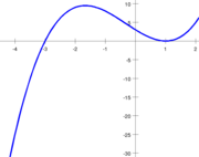
Example
Suppose that we are seeking a zero of the function defined by f(x) = (x + 3)(x − 1)2. We take [a0, b0] = [−4, 4/3] as our initial interval. We have f(a0) = −25 and f(b0) = 0.48148 (all numbers in this section are rounded), so the conditions f(a0) f(b0) < 0 and |f(b0)| ≤ |f(a0)| are satisfied.- In the first iteration, we use linear interpolation between (b−1, f(b−1)) = (a0, f(a0)) = (−4, −25) and (b0, f(b0)) = (1.33333, 0.48148), which yields s = 1.23256. This lies between (3a0 + b0) / 4 and b0, so this value is accepted. Furthermore, f(1.23256) = 0.22891, so we set a1 = a0 and b1 = s = 1.23256.
- In the second iteration, we use inverse quadratic interpolation between (a1, f(a1)) = (−4, −25) and (b0, f(b0)) = (1.33333, 0.48148) and (b1, f(b1)) = (1.23256, 0.22891). This yields 1.14205, which lies between (3a1 + b1) / 4 and b1. Furthermore, the inequality |1.14205 − b1| ≤ |b0 − b−1| / 2 is satisfied, so this value is accepted. Furthermore, f(1.14205) = 0.083582, so we set a2 = a1 and b2 = 1.14205.
- In the third iteration, we use inverse quadratic interpolation between (a2, f(a2)) = (−4, −25) and (b1, f(b1)) = (1.23256, 0.22891) and (b2, f(b2)) = (1.14205, 0.083582). This yields 1.09032, which lies between (3a2 + b2) / 4 and b2. But here Brent's additional condition kicks in: the inequality |1.09032 − b2| ≤ |b1 − b0| / 2 is not satisfied, so this value is rejected. Instead, the midpoint m = −1.42897 of the interval [a2, b2] is computed. We have f(m) = 9.26891, so we set a3 = a2 and b3 = −1.42897.
- In the fourth iteration, we use inverse quadratic interpolation between (a3, f(a3)) = (−4, −25) and (b2, f(b2)) = (1.14205, 0.083582) and (b3, f(b3)) = (−1.42897, 9.26891). This yields 1.15448, which is not in the interval between (3a3 + b3) / 4 and b3). Hence, it is replaced by the midpoint m = −2.71449. We have f(m) = 3.93934, so we set a4 = a3 and b4 = −2.71449.
- In the fifth iteration, inverse quadratic interpolation yields −3.45500, which lies in the required interval. However, the previous iteration was a bisection step, so the inequality |−3.45500 − b4| ≤ |b4 − b3| / 2 need to be satisfied. This inequality is false, so we use the midpoint m = −3.35724. We have f(m) = −6.78239, so m becomes the new contrapoint (a5 = −3.35724) and the iterate remains the same (b5 = b4).
- In the sixth iteration, we cannot use inverse quadratic interpolation because b5 = b4. Hence, we use linear interpolation between (a5, f(a5)) = (−3.35724, −6.78239) and (b5, f(b5)) = (−2.71449, 3.93934). The result is s = −2.95064, which satisfies all the conditions. But since the iterate did not change in the previous step, we reject this result and fall back to bisection. We update s = -3.03587, and f(s) = -0.58418.
- In the seventh iteration, we can again use inverse quadratic interpolation. The result is s = −3.00219, which satisfies all the conditions. Now, f(s) = −0.03515, so we set a7 = b6 and b7 = −3.00219 (a7 and b7 are exchanged so that the condition |f(b7)| ≤ |f(a7)| is satisfied). (Correct : linear interpolation s = -2.99436, f(s) = 0.089961)
- In the eighth iteration, we cannot use inverse quadratic interpolation because a7 = b6. Linear interpolation yields s = −2.99994, which is accepted. (Correct : s = -2.9999, f(s) = 0.0016)
- In the following iterations, the root x = −3 is approached rapidly: b9 = −3 + 6·10−8 and b10 = −3 − 3·10−15. (Correct : Iter 9 : f(s) = -1.4E-07, Iter 10 : f(s) = 6.96E-12)
Implementations
- Brent (1973) published an Algol 60ALGOL 60ALGOL 60 is a member of the ALGOL family of computer programming languages. It gave rise to many other programming languages, including BCPL, B, Pascal, Simula, C, and many others. ALGOL 58 introduced code blocks and the begin and end pairs for delimiting them...
implementation. - NetlibNetlibNetlib is a repository of software for scientific computing maintained by AT&T, Bell Laboratories, the University of Tennessee and Oak Ridge National Laboratory. Netlib comprises a large number of separate programs and libraries...
contains a Fortran translation of this implementation with slight modifications. - The PARI/GPPARI/GPPARI/GP is a computer algebra system with the main aim of facilitating number theory computations. It is free software; versions 2.1.0 and higher are distributed under the GNU General Public License...
method solve implements the method. - Other implementations of the algorithm (in C++, C, and Fortran) can be found in the Numerical RecipesNumerical RecipesNumerical Recipes is the generic title of a series of books on algorithms and numerical analysis by William H. Press, Saul Teukolsky, William Vetterling and Brian Flannery. In various editions, the books have been in print since 1986...
books. - The Apache Commons Math library implements the algorithm in JavaJavaJava is an island of Indonesia. With a population of 135 million , it is the world's most populous island, and one of the most densely populated regions in the world. It is home to 60% of Indonesia's population. The Indonesian capital city, Jakarta, is in west Java...
.
External links
- Wikipedia Brent algorithm - Implementation in Borland Delphi (console application) by vpapanik - 24 Aug 2010
- Wikipedia Brent example - Solution Table by vpapanik - 8 Sep 2009
- zeroin.f at NetlibNetlibNetlib is a repository of software for scientific computing maintained by AT&T, Bell Laboratories, the University of Tennessee and Oak Ridge National Laboratory. Netlib comprises a large number of separate programs and libraries...
. - Module for Brent's Method by John H. Mathews
- Open source Excel VBA functions and examples, including step by step evaluation of the example problem