

Time-frequency analysis
Encyclopedia
In signal processing
, time–frequency analysis comprises those techniques that study a signal in both the time and frequency domains simultaneously, using various time–frequency representations. Rather than viewing a 1-dimensional signal (a function, real or complex-valued, whose domain is the real line) and some transform (another function whose domain is the real line, obtained from the original via some transform), time–frequency analysis studies a two-dimensional signal – a function whose domain is the two-dimensional real plane, obtained from the signal via a time–frequency transform.
The mathematical motivation for this study is that functions and their transform representation are often tightly connected, and they can be understood better by studying them jointly, as a two-dimensional object, rather than separately. A simple example is that the 4-fold periodicity of the Fourier transform
– and the fact that two-fold Fourier transform reverses direction – can be interpreted by considering the Fourier transform as a 90° rotation in the associated time–frequency plane: 4 such rotations yield the identity, and 2 such rotation simply reverse direction (reflection through the origin).
The practical motivation for time–frequency analysis is that classical Fourier analysis assumes that signals are infinite in time or periodic, while many signals in practice are of short duration, and change substantially over their duration. For example, traditional musical instruments do not produce infinite duration sinusoids, but instead begin with an attack, then gradually decay. This is poorly represented by traditional methods, which motivates time–frequency analysis.
One of the most basic forms of time–frequency analysis is the short-time Fourier transform
(STFT), but more sophisticated techniques have been developed, notably wavelet
s.
, time–frequency analysis is a body of techniques and methods used for characterizing and manipulating signals whose statistics vary in time, such as transient signals.
It is a generalization and refinement of Fourier analysis, for the case when the signal frequency characteristics are varying with time. Since many signals of interest – such as speech, music, images, and medical signals – have changing frequency characteristics, time–frequency analysis has broad scope of applications.
Whereas the technique of the Fourier transform
can be extended to obtain the frequency spectrum of any slowly growing locally integrable signal, this approach requires a complete description of the signal's behavior over all time. Indeed, one can think of points in the (spectral) frequency domain as smearing together information from across the entire time domain. While mathematically elegant, such a technique is not appropriate for analyzing a signal with indeterminate future behavior. For instance, one must presuppose some degree of indeterminate future behavior in any telecommunications systems to achieve non-zero entropy (if one already knows what the other person will say one cannot learn anything).
To harness the power of a frequency representation without the need of a complete characterization in the time domain, one first obtains a time–frequency distribution of the signal, which represents the signal in both the time and frequency domains simultaneously. In such a representation the frequency domain will only reflect the behavior of a temporally localized version of the signal. This enables one to talk sensibly about signals whose component frequencies vary in time.
For instance rather than using tempered distributions to globally transform the following function into the frequency domain one could instead use these methods to describe it as a signal with a time varying frequency.
Signal processing
Signal processing is an area of systems engineering, electrical engineering and applied mathematics that deals with operations on or analysis of signals, in either discrete or continuous time...
, time–frequency analysis comprises those techniques that study a signal in both the time and frequency domains simultaneously, using various time–frequency representations. Rather than viewing a 1-dimensional signal (a function, real or complex-valued, whose domain is the real line) and some transform (another function whose domain is the real line, obtained from the original via some transform), time–frequency analysis studies a two-dimensional signal – a function whose domain is the two-dimensional real plane, obtained from the signal via a time–frequency transform.
The mathematical motivation for this study is that functions and their transform representation are often tightly connected, and they can be understood better by studying them jointly, as a two-dimensional object, rather than separately. A simple example is that the 4-fold periodicity of the Fourier transform
Fourier transform
In mathematics, Fourier analysis is a subject area which grew from the study of Fourier series. The subject began with the study of the way general functions may be represented by sums of simpler trigonometric functions...
– and the fact that two-fold Fourier transform reverses direction – can be interpreted by considering the Fourier transform as a 90° rotation in the associated time–frequency plane: 4 such rotations yield the identity, and 2 such rotation simply reverse direction (reflection through the origin).
The practical motivation for time–frequency analysis is that classical Fourier analysis assumes that signals are infinite in time or periodic, while many signals in practice are of short duration, and change substantially over their duration. For example, traditional musical instruments do not produce infinite duration sinusoids, but instead begin with an attack, then gradually decay. This is poorly represented by traditional methods, which motivates time–frequency analysis.
One of the most basic forms of time–frequency analysis is the short-time Fourier transform
Short-time Fourier transform
The short-time Fourier transform , or alternatively short-term Fourier transform, is a Fourier-related transform used to determine the sinusoidal frequency and phase content of local sections of a signal as it changes over time....
(STFT), but more sophisticated techniques have been developed, notably wavelet
Wavelet
A wavelet is a wave-like oscillation with an amplitude that starts out at zero, increases, and then decreases back to zero. It can typically be visualized as a "brief oscillation" like one might see recorded by a seismograph or heart monitor. Generally, wavelets are purposefully crafted to have...
s.
Need for a time–frequency approach
In signal processingSignal processing
Signal processing is an area of systems engineering, electrical engineering and applied mathematics that deals with operations on or analysis of signals, in either discrete or continuous time...
, time–frequency analysis is a body of techniques and methods used for characterizing and manipulating signals whose statistics vary in time, such as transient signals.
It is a generalization and refinement of Fourier analysis, for the case when the signal frequency characteristics are varying with time. Since many signals of interest – such as speech, music, images, and medical signals – have changing frequency characteristics, time–frequency analysis has broad scope of applications.
Whereas the technique of the Fourier transform
Fourier transform
In mathematics, Fourier analysis is a subject area which grew from the study of Fourier series. The subject began with the study of the way general functions may be represented by sums of simpler trigonometric functions...
can be extended to obtain the frequency spectrum of any slowly growing locally integrable signal, this approach requires a complete description of the signal's behavior over all time. Indeed, one can think of points in the (spectral) frequency domain as smearing together information from across the entire time domain. While mathematically elegant, such a technique is not appropriate for analyzing a signal with indeterminate future behavior. For instance, one must presuppose some degree of indeterminate future behavior in any telecommunications systems to achieve non-zero entropy (if one already knows what the other person will say one cannot learn anything).
To harness the power of a frequency representation without the need of a complete characterization in the time domain, one first obtains a time–frequency distribution of the signal, which represents the signal in both the time and frequency domains simultaneously. In such a representation the frequency domain will only reflect the behavior of a temporally localized version of the signal. This enables one to talk sensibly about signals whose component frequencies vary in time.
For instance rather than using tempered distributions to globally transform the following function into the frequency domain one could instead use these methods to describe it as a signal with a time varying frequency.
-
Once such a representation has been generated other techniques in time–frequency analysis may then be applied to the signal in order to extract information from the signal, to separate the signal from noise or interfering signals, etc.
Diversity of time–frequency formulations
There are several different ways to formulate a valid time–frequency distribution function, resulting in several well-known time–frequency distributions, such as:
- Short-time Fourier transformShort-time Fourier transformThe short-time Fourier transform , or alternatively short-term Fourier transform, is a Fourier-related transform used to determine the sinusoidal frequency and phase content of local sections of a signal as it changes over time....
(including the Gabor transformGabor transformThe Gabor transform, named after Dennis Gabor, is a special case of the short-time Fourier transform. It is used to determine the sinusoidal frequency and phase content of local sections of a signal as it changes over time...
), - Wavelet transform,
- Bilinear time–frequency distribution function (Wigner distribution functionWigner distribution functionThe Wigner distribution function was first proposed to account for quantum corrections to classical statistical mechanics in 1932 by Eugene Wigner, cf. Wigner quasi-probability distribution....
), - Modified Wigner distribution functionModified Wigner distribution functionThe Wigner distribution was first proposed for corrections to classical statistical mechanics in 1932 by Eugene Wigner. The Wigner distribution, or Wigner–Ville distribution for analytic signals, also has applications in time frequency analysis...
, Gabor–Wigner distribution function, and so on (see Gabor–Wigner transform).
More information about the history and the motivation of development of time–frequency distribution can be found in the entry Time–frequency representation.
Ideal TF distribution function
A time–frequency distribution function ideally has the following properties:
- High clarity to make it easier to be analyzed and interpreted.
- No cross-term to avoid confusing real components from artefacts or noise.
- A list of desirable mathematical properties to ensure such methods benefit real-life application.
- Lower computational complexity to ensure the time needed to represent and process a signal on a time–frequency plane allows real-time implementations.
Below is a brief comparison of some selected time–frequency distribution functions.
Clarity Cross-term Good mathematical properties Computational complexity Gabor transform Worst No Worst Low Wigner distribution function Best Yes Best High Gabor-Wigner distribution function Good Almost eliminated Good High
To analyze the signals well, choosing an appropriate time–frequency distribution function is important. Which time–frequency distribution function should be used depends on the application being considered, as shown by reviewing a list of applications. The high clarity of the Wigner distribution function (WDF) obtained for some signals is due to the auto-correlation function inherent in its formulation; however, the latter also causes the cross-term problem. Therefore, if we want to analyze a single-term signal, using the WDF may be the best approach; if the signal is composed of multiple components, some other methods like the Gabor transform, Gabor-Wigner distribution or Modified B-Distribution functions may be better choices.
To illustrate this, we observe that by Fourier analysis, we can’t recognize the two signals and
and  below.
-

-
Thanks to the time–frequency analysis approach, we can still solve this problem of correctly identifying the two different signals.
Signal processing applications
The following applications need not only the time–frequency distribution functions but also some operations to the signal. The Linear canonical transform (LCT) is really helpful. By LCTs, the shape and location on the time–frequency plane of a signal can be in the arbitrary form that we want it to be. For example, the LCTs can shift the time–frequency distribution to any location, dilate it in the horizontal and vertical direction without changing its area on the plane, shear (or twist) it, and rotate it (Fractional Fourier transformFractional Fourier transformIn mathematics, in the area of harmonic analysis, the fractional Fourier transform is a linear transformation generalizing the Fourier transform. It can be thought of as the Fourier transform to the n-th power where n need not be an integer — thus, it can transform a function to an...
). This powerful operation, LCT, make it more flexible to analyze and apply the time–frequency distributions. Here we list some applications of time–frequency analysis.
Instantaneous frequency estimation
The definition of instantaneous frequency is the time rate of change of phase, or
where is the instantaneous phaseInstantaneous phaseThe notions of Instantaneous Phase and Instantaneous Frequency are important concepts in Signal Processing that occur in the context of the representation and analysis of time-varying signals....
of a signal. We can know the instantaneous frequency from the time–frequency plane directly if the image is clear enough. Because the high clarity is critical, we often use WDF to analyze it.
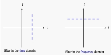
TF filtering and signal decomposition
The goal of filter design is to remove the undesired component of a signal. Conventionally, we can just filter in the time domain or in the frequency domain individually as shown below.
The filtering methods mentioned above can’t work well for every signal which may overlap in the time domain or in the frequency domain. By using the time–frequency distribution function, we can filter in the Euclidian time–frequency domain or in the fractional domain by employing the fractional Fourier transformFractional Fourier transformIn mathematics, in the area of harmonic analysis, the fractional Fourier transform is a linear transformation generalizing the Fourier transform. It can be thought of as the Fourier transform to the n-th power where n need not be an integer — thus, it can transform a function to an...
. An example is shown below.
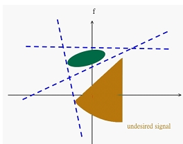
Filter design in time–frequency analysis always deals with signals composed of multiple components, so one cannot use WDF due to cross-term. The Gabor transform, Gabor-Wigner distribution function, or Cohen's class distribution function may be better choices.
The concept of signal decomposition relates to the need to separate one component from the others in a signal; this can be achieved through a filtering operation which require a filter design stage. Such filtering is traditionally done in the time domain or in the frequency domain; however, this may not be possible in the case of non-stationary signals that are multicomponent as such components could overlap in both the time domain and also in the frequency domain; as a consequence, the only possible way to achieve component separation and therefore a signal decomposition is to implement a time–frequency filter.
Sampling theory
By the Nyquist–Shannon sampling theoremNyquist–Shannon sampling theoremThe Nyquist–Shannon sampling theorem, after Harry Nyquist and Claude Shannon, is a fundamental result in the field of information theory, in particular telecommunications and signal processing. Sampling is the process of converting a signal into a numeric sequence...
, we can conclude that the minimum number of sampling points without aliasingAliasingIn signal processing and related disciplines, aliasing refers to an effect that causes different signals to become indistinguishable when sampled...
is equivalent to the area of the time–frequency distribution of a signal. (This is actually just an approximation, because the TF area of any signal is infinite.) Below is an example before and after we combine the sampling theory with the time–frequency distribution:
It is noticeable that the number of sampling points decreases after we apply the time–frequency distribution.
When we use the WDF, there might be the cross-term problem (also called interference). On the other hand, using Gabor transformGabor transformThe Gabor transform, named after Dennis Gabor, is a special case of the short-time Fourier transform. It is used to determine the sinusoidal frequency and phase content of local sections of a signal as it changes over time...
causes an improvement in the clarity and readability of the representation, therefore improving its interpretation and application to practical problems.
Consequently, when the signal we tend to sample is composed of single component, we use the WDF; however, if the signal consists of more than one component, using the Gabor transform, Gabor-Wigner distribution function, or other reduced interference TFDs may achieve better results.
The Balian–Low theorem formalizes this, and provides a bound on the minimum number of time–frequency samples needed.
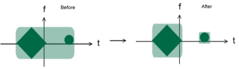
Modulation and multiplexing
Conventionally, the operation of modulationModulationIn electronics and telecommunications, modulation is the process of varying one or more properties of a high-frequency periodic waveform, called the carrier signal, with a modulating signal which typically contains information to be transmitted...
and multiplexingMultiplexingThe multiplexed signal is transmitted over a communication channel, which may be a physical transmission medium. The multiplexing divides the capacity of the low-level communication channel into several higher-level logical channels, one for each message signal or data stream to be transferred...
concentrates in time or in frequency, separately. By taking advantage of the time–frequency distribution, we can make it more efficient to modulate and multiplex. All we have to do is to fill up the time–frequency plane. We present an example as below.
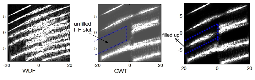
As illustrated in the upper example, using the WDF is not smart since the serious cross-term problem make it difficult to multiplex and modulation.
Electromagnetic wave propagation
We can represent an electromagnetic wave in the form of a 2 by 1 matrix
-

which is similar to the time–frequency plane. When electromagnetic wave propagates through free-space, the Fresnel diffractionFresnel diffractionIn optics, the Fresnel diffraction equation for near-field diffraction, is an approximation of Kirchhoff-Fresnel diffraction that can be applied to the propagation of waves in the near field....
occurs. We can operate with the 2 by 1 matrix
-
by LCT with parameter matrix
-

where z is the propagation distance and is the wavelength. When electromagnetic wave pass through a spherical lens or be reflected by a disk, the parameter matrix should be
-
and
-
respectively, where ƒ is the focal length of the lens and R is the radius of the disk. These corresponding results can be obtained from
-

Optics, acoustics, and biomedicine
LightLightLight or visible light is electromagnetic radiation that is visible to the human eye, and is responsible for the sense of sight. Visible light has wavelength in a range from about 380 nanometres to about 740 nm, with a frequency range of about 405 THz to 790 THz...
is a kind of electromagnetic wave, so we apply the time–frequency analysis to optics in the same way as to electromagnetic wave propagation. In the same way, a characteristic of acoustic signals is that, often, its frequency varies really severely with time. Because the acoustic signals usually contain a lot of data, it is suitable to use simpler TFDs such as the Gabor transform to analyze the acoustic signals due to the lower computational complexity. If speed is not an issue, then a detailed comparison with well defined criteria should be made before selecting a particular TFD. Another approach is to define a signal dependent TFD that is adapted to the data.
In biomedicine, one can use time–frequency distribution to analyze the electromyographyElectromyographyElectromyography is a technique for evaluating and recording the electrical activity produced by skeletal muscles. EMG is performed using an instrument called an electromyograph, to produce a record called an electromyogram. An electromyograph detects the electrical potential generated by muscle...
(EMG), ElectroencephalographyElectroencephalographyElectroencephalography is the recording of electrical activity along the scalp. EEG measures voltage fluctuations resulting from ionic current flows within the neurons of the brain...
(EEG), ElectrocardiogramElectrocardiogramElectrocardiography is a transthoracic interpretation of the electrical activity of the heart over a period of time, as detected by electrodes attached to the outer surface of the skin and recorded by a device external to the body...
(ECG) or otoacoustic emissions (OAEs).
History
Early work in time–frequency analysis can be seen in the Haar waveletHaar waveletIn mathematics, the Haar wavelet is a certain sequence of rescaled "square-shaped" functions which together form a wavelet family or basis. Wavelet analysis is similar to Fourier analysis in that it allows a target function over an interval to be represented in terms of an orthonormal function basis...
s (1909) of Alfréd HaarAlfréd HaarAlfréd Haar was a Jewish Hungarian mathematician. In 1904 he began to study at the University of Göttingen. His doctorate was supervised by David Hilbert. The Haar measure, Haar wavelet, and Haar transform are named in his honor....
, though these were not significantly applied to signal processing. More substantial work was undertaken by Dennis GaborDennis GaborDennis Gabor CBE, FRS was a Hungarian-British electrical engineer and inventor, most notable for inventing holography, for which he later received the 1971 Nobel Prize in Physics....
, such as Gabor atoms (1947), an early form of waveletWaveletA wavelet is a wave-like oscillation with an amplitude that starts out at zero, increases, and then decreases back to zero. It can typically be visualized as a "brief oscillation" like one might see recorded by a seismograph or heart monitor. Generally, wavelets are purposefully crafted to have...
s, and the Gabor transformGabor transformThe Gabor transform, named after Dennis Gabor, is a special case of the short-time Fourier transform. It is used to determine the sinusoidal frequency and phase content of local sections of a signal as it changes over time...
, a modified short-time Fourier transformShort-time Fourier transformThe short-time Fourier transform , or alternatively short-term Fourier transform, is a Fourier-related transform used to determine the sinusoidal frequency and phase content of local sections of a signal as it changes over time....
. The Wigner–Ville distribution (Ville 1948, in a signal processing context) was another foundational step.
Particularly in the 1930s and 1940s, early time–frequency analysis developed in concert with quantum mechanicsQuantum mechanicsQuantum mechanics, also known as quantum physics or quantum theory, is a branch of physics providing a mathematical description of much of the dual particle-like and wave-like behavior and interactions of energy and matter. It departs from classical mechanics primarily at the atomic and subatomic...
(Wigner developed the Wigner–Ville distribution in 1932 in quantum mechanics, and Gabor was influenced by quantum mechanics – see Gabor atom); this is reflected in the shared mathematics of the position-momentum plane and the time–frequency plane – as in the Heisenberg uncertainty principle (quantum mechanics) and the Gabor limit (time–frequency analysis), ultimately both reflecting a symplectic structure.
An early practical motivation for time–frequency analysis was the development of radar – see ambiguity function.
See also history of wavelets.
See also
- WaveletWaveletA wavelet is a wave-like oscillation with an amplitude that starts out at zero, increases, and then decreases back to zero. It can typically be visualized as a "brief oscillation" like one might see recorded by a seismograph or heart monitor. Generally, wavelets are purposefully crafted to have...
- Time–frequency analysis for music signal
- Wavelet
-
-
-
-
-
-
-
- Short-time Fourier transform
