Home Discussion Topics Dictionary Almanac

Signup Login

Step response

Discussion

Ask a question about 'Step response'

Start a new discussion about 'Step response'

Answer questions from other users

Full Discussion Forum

Encyclopedia

The step response of a system in a given initial state consists of the time evolution of its outputs when its control inputs are Heaviside step function

Heaviside step function

The Heaviside step function, or the unit step function, usually denoted by H , is a discontinuous function whose value is zero for negative argument and one for positive argument....

s. In electronic engineering

Electronic engineering

Electronics engineering, also referred to as electronic engineering, is an engineering discipline where non-linear and active electrical components such as electron tubes, and semiconductor devices, especially transistors, diodes and integrated circuits, are utilized to design electronic...

and control theory

Control theory

Control theory is an interdisciplinary branch of engineering and mathematics that deals with the behavior of dynamical systems. The desired output of a system is called the reference...

, step response is the time behaviour of the outputs of a general system

System

System is a set of interacting or interdependent components forming an integrated whole....

when its inputs change from zero to one in a very short time. The concept can be extended to the abstract mathematical notion of a dynamical system

Dynamical system

A dynamical system is a concept in mathematics where a fixed rule describes the time dependence of a point in a geometrical space. Examples include the mathematical models that describe the swinging of a clock pendulum, the flow of water in a pipe, and the number of fish each springtime in a...

using an evolution parameter.

From a practical standpoint, knowing how the system responds to a sudden input is important because large and possibly fast deviations from the long term steady state may have extreme effects on the component itself and on other portions of the overall system dependent on this component. In addition, the overall system cannot act until the component's output settles down to some vicinity of its final state, delaying the overall system response. Formally, knowing the step response of a dynamical system gives information on the stability

Stability theory

In mathematics, stability theory addresses the stability of solutions of differential equations and of trajectories of dynamical systems under small perturbations of initial conditions...

of such a system, and on its ability to reach one stationary state when starting from another.

Time domain versus frequency domain

Instead of frequency response, system performance may be specified in terms of parameters describing time-dependence of response. The step response can be described by the following quantities related to its time behavior,

overshoot
Overshoot (signal)
In signal processing, control theory, electronics, and mathematics, overshoot is when a signal or function exceeds its target. It arises especially in the step response of bandlimited systems such as low-pass filters...
rise time
Rise time
In electronics, when describing a voltage or current step function, rise time refers to the time required for a signal to change from a specified low value to a specified high value...
settling time
Settling time
The settling time of an amplifier or other output device is the time elapsed from the application of an ideal instantaneous step input to the time at which the amplifier output has entered and remained within a specified error band, usually symmetrical about the final value.Settling time includes a...
ringing
Ringing (signal)
In electronics, signal processing, and video, ringing is unwanted oscillation of a signal, particularly in the step response...

In the case of linear

Linear

In mathematics, a linear map or function f is a function which satisfies the following two properties:* Additivity : f = f + f...

dynamic systems, much can be inferred about the system from these characteristics. Below the step response of a simple two-pole amplifier is presented, and some of these terms are illustrated.

Step response of feedback amplifiers

This section describes the step response of a simple negative feedback amplifier shown in Figure 1. The feedback amplifier consists of a main open-loop amplifier of gain A_OL and a feedback loop governed by a feedback factor β. This feedback amplifier is analyzed to determine how its step response depends upon the time constants governing the response of the main amplifier, and upon the amount of feedback used.

Analysis

A negative feedback amplifier has gain given by (see negative feedback amplifier):

where A_OL = open-loop gain, A_FB = closed-loop gain (the gain with negative feedback present) and β = feedback factor. The step response of such an amplifier is easily handled in the case that the open-loop gain has two poles (two time constant

Time constant

In physics and engineering, the time constant, usually denoted by the Greek letter \tau , is the risetime characterizing the response to a time-varying input of a first-order, linear time-invariant system.Concretely, a first-order LTI system is a system that can be modeled by a single first order...

s, τ₁, τ₂), that is, the open-loop gain is given by:

with zero-frequency gain A₀ and angular frequency ω = 2πf, which leads to the closed-loop gain:

•

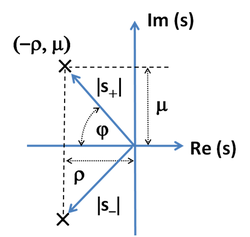
The time dependence of the amplifier is easy to discover by switching variables to s = jω, whereupon the gain becomes:

•

The poles of this expression (that is, the zeros of the denominator) occur at:

which shows for large enough values of βA₀ the square root becomes the square root of a negative number, that is the square root becomes imaginary, and the pole positions are complex conjugate numbers, either s₊ or s₋; see Figure 2:

with

and

Using polar coordinates with the magnitude of the radius to the roots given by |s| (Figure 2):

and the angular coordinate φ is given by:

Tables of Laplace transforms show that the time response of such a system is composed of combinations of the two functions:

which is to say, the solutions are damped oscillations in time. In particular, the unit step response of the system is:

Notice that the damping of the response is set by ρ, that is, by the time constants of the open-loop amplifier. In contrast, the frequency of oscillation is set by μ, that is, by the feedback parameter through βA₀. Because ρ is a sum of reciprocals of time constants, it is interesting to notice that ρ is dominated by the shorter of the two.

Results

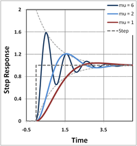
Figure 3 shows the time response to a unit step input for three values of the parameter μ. It can be seen that the frequency of oscillation increases with μ, but the oscillations are contained between the two asymptotes set by the exponentials [ 1 − exp (−ρt) ] and [ 1 + exp(−ρt) ]. These asymptotes are determined by ρ and therefore by the time constants of the open-loop amplifier, independent of feedback.

The phenomena of oscillation about final value is called ringing
Ringing (signal)
In electronics, signal processing, and video, ringing is unwanted oscillation of a signal, particularly in the step response...

. The overshoot
Overshoot (signal)
In signal processing, control theory, electronics, and mathematics, overshoot is when a signal or function exceeds its target. It arises especially in the step response of bandlimited systems such as low-pass filters...

is the maximum swing above final value, and clearly increases with μ. Likewise, the undershoot is the minimum swing below final value, again increasing with μ. The settling time
Settling time
The settling time of an amplifier or other output device is the time elapsed from the application of an ideal instantaneous step input to the time at which the amplifier output has entered and remained within a specified error band, usually symmetrical about the final value.Settling time includes a...

is the time for departures from final value to sink below some specified level, say 10% of final value.

The dependence of settling time upon μ is not obvious, and the approximation of a two-pole system probably is not accurate enough to make any real-world conclusions about feedback dependence of settling time. However, the asymptotes [ 1 − exp (−ρt) ] and [ 1 + exp (−ρt) ] clearly impact settling time, and they are controlled by the time constants of the open-loop amplifier, particularly the shorter of the two time constants. That suggests that a specification on settling time must be met by appropriate design of the open-loop amplifier.

The two major conclusions from this analysis are:

Feedback controls the amplitude of oscillation about final value for a given open-loop amplifier and given values of open-loop time constants, τ₁ and τ₂.
The open-loop amplifier decides settling time. It sets the time scale of Figure 3, and the faster the open-loop amplifier, the faster this time scale.

As an aside, it may be noted that real-world departures from this linear two-pole model occur due to two major complications: first, real amplifiers have more than two poles, as well as zeros; and second, real amplifiers are nonlinear, so their step response changes with signal amplitude.

Control of overshoot

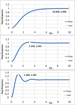
How overshoot may be controlled by appropriate parameter choices is discussed next.

Using the equations above, the amount of overshoot can be found by differentiating the step response and finding its maximum value. The result for maximum step response S_max is:

The final value of the step response is 1, so the exponential is the actual overshoot itself. It is clear the overshoot is zero if μ = 0, which is the condition:

This quadratic is solved for the ratio of time constants by setting x = ( τ₁ / τ₂ )^{1 / 2} with the result

Because β A₀ >> 1, the 1 in the square root can be dropped, and the result is

In words, the first time constant must be much larger than the second. To be more adventurous than a design allowing for no overshoot we can introduce a factor α in the above relation:

and let α be set by the amount of overshoot that is acceptable.

Figure 4 illustrates the procedure. Comparing the top panel (α = 4) with the lower panel (α = 0.5) shows lower values for α increase the rate of response, but increase overshoot. The case α = 2 (center panel) is the maximally flat design that shows no peaking in the Bode gain vs. frequency plot

Bode plot

A Bode plot is a graph of the transfer function of a linear, time-invariant system versus frequency, plotted with a log-frequency axis, to show the system's frequency response...

. That design has the rule of thumb

Rule of thumb

A rule of thumb is a principle with broad application that is not intended to be strictly accurate or reliable for every situation. It is an easily learned and easily applied procedure for approximately calculating or recalling some value, or for making some determination...

built-in safety margin to deal with non-ideal realities like multiple poles (or zeros), nonlinearity (signal amplitude dependence) and manufacturing variations, any of which can lead to too much overshoot. The adjustment of the pole separation (that is, setting α) is the subject of frequency compensation

Frequency compensation

In electrical engineering, frequency compensation is a technique used in amplifiers, and especially in amplifiers employing negative feedback. It usually has two primary goals: To avoid the unintentional creation of positive feedback, which will cause the amplifier to oscillate, and to control...

, and one such method is pole splitting

Pole splitting

Pole splitting is a phenomenon exploited in some forms of frequency compensation used in an electronic amplifier. When a capacitor is introduced between the input and output sides of the amplifier with the intention of moving the pole lowest in frequency to lower frequencies, pole splitting causes...

.

Control of settling time

The amplitude of ringing in the step response in Figure 3 is governed by the damping factor exp ( −ρ t ). That is, if we specify some acceptable step response deviation from final value, say Δ, that is:

this condition is satisfied regardless of the value of β A_OL provided the time is longer than the settling time, say t_S, given by:

where the approximation τ₁ >> τ₂ is applicable because of the overshoot control condition, which makes τ₁ = αβA_OL τ₂. Often the settling time condition is referred to by saying the settling period is inversely proportional to the unity gain bandwidth, because 1/(2π τ₂) is close to this bandwidth for an amplifier with typical dominant pole compensation. However, this result is more precise than this rule of thumb

Rule of thumb

A rule of thumb is a principle with broad application that is not intended to be strictly accurate or reliable for every situation. It is an easily learned and easily applied procedure for approximately calculating or recalling some value, or for making some determination...

. As an example of this formula, if Δ = 1/e⁴ = 1.8 %, the settling time condition is t_S = 8 τ₂.

In general, control of overshoot sets the time constant ratio, and settling time t_S sets τ₂.

Phase margin

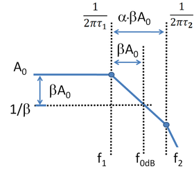
Next, the choice of pole ratio τ₁/τ₂ is related to the phase margin of the feedback amplifier. The procedure outlined in the Bode plot article is followed. Figure 5 is the Bode gain plot for the two-pole amplifier in the range of frequencies up to the second pole position. The assumption behind Figure 5 is that the frequency f_0 dB lies between the lowest pole at f₁ = 1/(2πτ₁) and the second pole at f₂ = 1/(2πτ₂). As indicated in Figure 5, this condition is satisfied for values of α ≥ 1.

Using Figure 5 the frequency (denoted by f_0 dB) is found where the loop gain βA₀ satisfies the unity gain or 0 dB condition, as defined by:

The slope of the downward leg of the gain plot is (20 dB/decade); for every factor of ten increase in frequency, the gain drops by the same factor:

The phase margin is the departure of the phase at f_0 dB from −180°. Thus, the margin is:

Because f_0 dB / f₁ = βA₀ >> 1, the term in f₁ is 90°. That makes the phase margin:

In particular, for case α = 1, φ_m = 45°, and for α = 2, φ_m = 63.4°. Sansen recommends α = 3, φ_m = 71.6° as a "good safety position to start with".

If α is increased by shortening τ₂, the settling time t_S also is shortened. If α is increased by lengthening τ₁, the settling time t_S is little altered. More commonly, both τ₁ and τ₂ change, for example if the technique of pole splitting

Pole splitting

Pole splitting is a phenomenon exploited in some forms of frequency compensation used in an electronic amplifier. When a capacitor is introduced between the input and output sides of the amplifier with the intention of moving the pole lowest in frequency to lower frequencies, pole splitting causes...

is used.

As an aside, for an amplifier with more than two poles, the diagram of Figure 5 still may be made to fit the Bode plots by making f₂ a fitting parameter, referred to as an "equivalent second pole" position.

Formal mathematical description

This section provides a formal mathematical definition of step response in terms of the abstract mathematical concept of a dynamical system

Dynamical system (definition)

The dynamical system concept is a mathematical formalization for any fixed "rule" which describes the time dependence of a point's position in its ambient space...

: all notations and assumptions required for the following description are listed here.

is the evolution parameter
Dynamical system (definition)
The dynamical system concept is a mathematical formalization for any fixed "rule" which describes the time dependence of a point's position in its ambient space...

of the system, called "time
Time
Time is a part of the measuring system used to sequence events, to compare the durations of events and the intervals between them, and to quantify rates of change such as the motions of objects....

" for the sake of simplicity,
is the state
Dynamical system (definition)
The dynamical system concept is a mathematical formalization for any fixed "rule" which describes the time dependence of a point's position in its ambient space...

of the system at time , called "output" for the sake of simplicity,
is the dynamical system evolution function
Dynamical system (definition)
The dynamical system concept is a mathematical formalization for any fixed "rule" which describes the time dependence of a point's position in its ambient space...

,
is the dynamical system initial state
Dynamical system (definition)
The dynamical system concept is a mathematical formalization for any fixed "rule" which describes the time dependence of a point's position in its ambient space...

,
is the Heaviside step function
Heaviside step function
The Heaviside step function, or the unit step function, usually denoted by H , is a discontinuous function whose value is zero for negative argument and one for positive argument....

Nonlinear dynamical system

For a general dynamical system, the step response is defined as follows:

It is the evolution function

Dynamical system (definition)

The dynamical system concept is a mathematical formalization for any fixed "rule" which describes the time dependence of a point's position in its ambient space...

when the control inputs (or source term

Linear differential equation

Linear differential equations are of the formwhere the differential operator L is a linear operator, y is the unknown function , and the right hand side ƒ is a given function of the same nature as y...

, or forcing inputs) are Heaviside functions: the notation emphasizes this concept showing H(t) as a subscript.

Linear dynamical system

For a linear

Linear system

A linear system is a mathematical model of a system based on the use of a linear operator.Linear systems typically exhibit features and properties that are much simpler than the general, nonlinear case....

time-invariant

Time-invariant system

A time-invariant system is one whose output does not depend explicitly on time.This property can be satisfied if the transfer function of the system is not a function of time except expressed by the input and output....

black box, let

for notational convenience: the step response can be obtained by convolution

Convolution

In mathematics and, in particular, functional analysis, convolution is a mathematical operation on two functions f and g, producing a third function that is typically viewed as a modified version of one of the original functions. Convolution is similar to cross-correlation...

of the Heaviside step function

Heaviside step function

The Heaviside step function, or the unit step function, usually denoted by H , is a discontinuous function whose value is zero for negative argument and one for positive argument....

control and the impulse response

Impulse response

In signal processing, the impulse response, or impulse response function , of a dynamic system is its output when presented with a brief input signal, called an impulse. More generally, an impulse response refers to the reaction of any dynamic system in response to some external change...

h(t) of the system itself

External links

Kuo power point slides; Chapter 7 especially