Simplex algorithm
Encyclopedia
In mathematical optimization
, Dantzig
's simplex algorithm (or simplex method) is a popular algorithm
for linear programming
.
The journal Computing in Science and Engineering listed it as one of the top 10 algorithms of the twentieth century.
The name of the algorithm is derived from the concept of a simplex
and was suggested by T. S. Motzkin
. Simplices are not actually used in the method, but one interpretation of it is that it operates on simplicial cone
s, and these become proper simplices with an additional constraint. The simplicial cones in question are the corners (i.e., the neighborhoods of the vertices) of a geometric object called polytope
. The shape of this polytope is defined by the constraints applied to the objective function.
 The simplex algorithm operates on linear programs in standard form, that is linear programming problems of the form,
with the variables of the problem,
  are the coefficients of the objective function, A, a p×n matrix and
  constants. There is a straightforward process to convert any linear program into one in standard form so this results in no loss of generality.
In geometric terms, the feasible region
is a (possibly unbounded) convex polytope
. There is a simple characterization of the extreme points or vertices of this polytope, namely is an extreme point if and only if the column vectors
  , where
 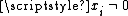 , are linearly independent
. In this context such a point is known as a basic feasible solution (BFS).
It can be shown that for a linear program in standard form, if the objective function has a minimum value on the feasible region then it has this value on (at least) one of the extreme points. This in itself reduces the problem to a finite computation since there are finite number of extreme points, however the number of extreme points is unmanageably large for all but the smallest linear programs.
It can also be shown that if an extreme point is not a minimum point of the objective function then there is an edge containing the point so that the objective function is strictly decreasing on the edge moving away from the point. If the edge is finite then the edge connects to another extreme point where the objective function has a smaller value, otherwise the objective function is unbounded below on the edge and the linear program has no solution. The simplex algorithm applies this insight by walking along edges of the polytope to extreme points with lower and lower objective values. This continues until the minimum value is reached or an unbounded edge is visited, concluding that the problem has no solution. The algorithm always terminates because the number of vertices in the polytope is finite; moreover since we jump between vertices always in the same direction (that of the objective function), we hope that the number of vertices visited will be small.
The solution of a linear program is accomplished in two steps. In the first step, known as Phase I, a starting extreme point is found. Depending on the nature of the program this may be trivial, but in general it can be solved by applying the simplex algorithm to a modified version of the original program. The possible results of Phase I are either a basic feasible solution is found or that the feasible region is empty. In the latter case the linear program is called infeasible. In the second step, Phase II, the simplex algorithm is applied using the basic feasible solution found in Phase I as a starting point. The possible results from Phase II are either an optimum basic feasible solution or an infinite edge on which the objective function is unbounded below.

a new variable, y1, is introduced with
The second equation may be used to eliminate x1 from the linear program. In this way, all lower bound constraints may be changed to nonnegativity restrictions.
Second, for each remaining inequality constraint, a new variable, called a slack variable, is introduced to change the constraint to an equality constraint. This variable represents the difference between the two sides of the inequality and is assumed to be nonnegative. For example the inequalities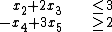
are replaced with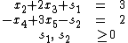
It is much easier to perform algebraic manipulation on inequalities in this form. In inequalities where ≥ appears such as the second one, some authors refer to the variable introduced as a surplus variable.
Third, each unrestricted variable is eliminated from the linear program. This can be done in two ways, one is by solving for the variable in one of the equations in which it appears and then eliminating the variable by substitution. The other is to replace the variable with the difference of two restricted variables. For example if z1 is unrestricted then write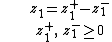
The equation may be used to eliminate z1 from the linear program.
When this process is complete the feasible region will be in the form
It is also useful to assume that the rank of A is the number of rows. This results in no loss of generality since otherwise either the system Ax >= b has redundant equations which can be dropped, or the system is inconsistent and the linear program has no solution.

The first row defines the objective function and the remaining rows specify the constraints. (Note, different authors use different conventions as to the exact layout.) If the columns of A can be rearranged so that it contains the identity matrix
of order p (the number of rows in A) then the tableau is said to be in canonical form. The variables corresponding to the columns of the identity matrix are called basic variables while the remaining variables are called nonbasic or free variables. If the nonbasic variables are assumed to be 0, then the values of the basic variables are easily obtained as entries in b and this solution is a basic feasible solution.
Conversely, given a basic feasible solution, the columns corresponding to the nonzero variables can be expanded to a nonsingular matrix. If the corresponding tableau is multiplied by the inverse of this matrix then the result is a tableau in canonical form.
Let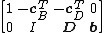
be a tableau in canonical form. Additional row-addition transformations can be applied to remove the coefficients cTB from the objective function. This process is called pricing out and results in a canonical tableau
where zB is the value of the objective function at the corresponding basic feasible solution. The updated coefficients, also known as relative cost coefficients, are the rates of change of the objective function with respect to the nonbasic variables.
If there is more than one column so that the entry in the objective row is positive then the choice of which one to add to the set of basic variables is somewhat arbitrary and several entering variable choice rules have been developed.
If all the entries in the objective row are less than or equal to 0 then no choice of entering variable can be made and the solution is in fact optimal. It is easily seen to be optimal since the objective row now corresponds to an equation of the form
Note that by changing the entering variable choice rule so that it selects a column where the entry in the objective row is negative, the algorithm is changed so that it finds the maximum of the objective function rather than the minimum.
Next, the pivot row must be selected so that all the other basic variables remain positive. A calculation shows that this occurs when the resulting value of the entering variable is at a minimum. In other words, if the pivot column is c, then the pivot row r is chosen so that
is the minimum over all r so that acr > 0. This is called the minimum ratio test. If there is more than one row for which the minimum is achieved then a dropping variable choice rule can be used to make the determination.
Optimization (mathematics)
In mathematics, computational science, or management science, mathematical optimization refers to the selection of a best element from some set of available alternatives....
, Dantzig
George Dantzig
George Bernard Dantzig was an American mathematical scientist who made important contributions to operations research, computer science, economics, and statistics....
's simplex algorithm (or simplex method) is a popular algorithm
Algorithm
In mathematics and computer science, an algorithm is an effective method expressed as a finite list of well-defined instructions for calculating a function. Algorithms are used for calculation, data processing, and automated reasoning...
for linear programming
Linear programming
Linear programming is a mathematical method for determining a way to achieve the best outcome in a given mathematical model for some list of requirements represented as linear relationships...
.
The journal Computing in Science and Engineering listed it as one of the top 10 algorithms of the twentieth century.
The name of the algorithm is derived from the concept of a simplex
Simplex
In geometry, a simplex is a generalization of the notion of a triangle or tetrahedron to arbitrary dimension. Specifically, an n-simplex is an n-dimensional polytope which is the convex hull of its n + 1 vertices. For example, a 2-simplex is a triangle, a 3-simplex is a tetrahedron,...
and was suggested by T. S. Motzkin
Theodore Motzkin
Theodore Samuel Motzkin was an Israeli-American mathematician.- Biography :Motzkin's father, Leo Motzkin, was a noted Russian Zionist leader.Motzkin received his Ph.D...
. Simplices are not actually used in the method, but one interpretation of it is that it operates on simplicial cone
Cone
A cone is a basic geometrical shape; see cone .Cone may also refer to:-Mathematics:*Cone , a family of morphisms resembling a geometric cone...
s, and these become proper simplices with an additional constraint. The simplicial cones in question are the corners (i.e., the neighborhoods of the vertices) of a geometric object called polytope
Polytope
In elementary geometry, a polytope is a geometric object with flat sides, which exists in any general number of dimensions. A polygon is a polytope in two dimensions, a polyhedron in three dimensions, and so on in higher dimensions...
. The shape of this polytope is defined by the constraints applied to the objective function.
Overview
- Minimize
- Subject to


with
the variables of the problem, are the coefficients of the objective function, A, a p×n matrix and constants. There is a straightforward process to convert any linear program into one in standard form so this results in no loss of generality.In geometric terms, the feasible region

is a (possibly unbounded) convex polytope
Convex polytope
A convex polytope is a special case of a polytope, having the additional property that it is also a convex set of points in the n-dimensional space Rn...
. There is a simple characterization of the extreme points or vertices of this polytope, namely
is an extreme point if and only if the column vectors , where , are linearly independentLinear independence
In linear algebra, a family of vectors is linearly independent if none of them can be written as a linear combination of finitely many other vectors in the collection. A family of vectors which is not linearly independent is called linearly dependent...
. In this context such a point is known as a basic feasible solution (BFS).
It can be shown that for a linear program in standard form, if the objective function has a minimum value on the feasible region then it has this value on (at least) one of the extreme points. This in itself reduces the problem to a finite computation since there are finite number of extreme points, however the number of extreme points is unmanageably large for all but the smallest linear programs.
It can also be shown that if an extreme point is not a minimum point of the objective function then there is an edge containing the point so that the objective function is strictly decreasing on the edge moving away from the point. If the edge is finite then the edge connects to another extreme point where the objective function has a smaller value, otherwise the objective function is unbounded below on the edge and the linear program has no solution. The simplex algorithm applies this insight by walking along edges of the polytope to extreme points with lower and lower objective values. This continues until the minimum value is reached or an unbounded edge is visited, concluding that the problem has no solution. The algorithm always terminates because the number of vertices in the polytope is finite; moreover since we jump between vertices always in the same direction (that of the objective function), we hope that the number of vertices visited will be small.
The solution of a linear program is accomplished in two steps. In the first step, known as Phase I, a starting extreme point is found. Depending on the nature of the program this may be trivial, but in general it can be solved by applying the simplex algorithm to a modified version of the original program. The possible results of Phase I are either a basic feasible solution is found or that the feasible region is empty. In the latter case the linear program is called infeasible. In the second step, Phase II, the simplex algorithm is applied using the basic feasible solution found in Phase I as a starting point. The possible results from Phase II are either an optimum basic feasible solution or an infinite edge on which the objective function is unbounded below.
Standard form
The transformation of a linear program to one in standard form may be accomplished as follows. First, for each variable with a lower bound other than 0, a new variable is introduced representing the difference between the variable and bound. The original variable can then be eliminated by substitution. For example, given the constrainta new variable, y1, is introduced with
The second equation may be used to eliminate x1 from the linear program. In this way, all lower bound constraints may be changed to nonnegativity restrictions.
Second, for each remaining inequality constraint, a new variable, called a slack variable, is introduced to change the constraint to an equality constraint. This variable represents the difference between the two sides of the inequality and is assumed to be nonnegative. For example the inequalities
are replaced with
It is much easier to perform algebraic manipulation on inequalities in this form. In inequalities where ≥ appears such as the second one, some authors refer to the variable introduced as a surplus variable.
Third, each unrestricted variable is eliminated from the linear program. This can be done in two ways, one is by solving for the variable in one of the equations in which it appears and then eliminating the variable by substitution. The other is to replace the variable with the difference of two restricted variables. For example if z1 is unrestricted then write
The equation may be used to eliminate z1 from the linear program.
When this process is complete the feasible region will be in the form
It is also useful to assume that the rank of A is the number of rows. This results in no loss of generality since otherwise either the system Ax >= b has redundant equations which can be dropped, or the system is inconsistent and the linear program has no solution.
Canonical tableaux
A linear program in standard form can be represented as a tableau of the formThe first row defines the objective function and the remaining rows specify the constraints. (Note, different authors use different conventions as to the exact layout.) If the columns of A can be rearranged so that it contains the identity matrix
Identity matrix
In linear algebra, the identity matrix or unit matrix of size n is the n×n square matrix with ones on the main diagonal and zeros elsewhere. It is denoted by In, or simply by I if the size is immaterial or can be trivially determined by the context...
of order p (the number of rows in A) then the tableau is said to be in canonical form. The variables corresponding to the columns of the identity matrix are called basic variables while the remaining variables are called nonbasic or free variables. If the nonbasic variables are assumed to be 0, then the values of the basic variables are easily obtained as entries in b and this solution is a basic feasible solution.
Conversely, given a basic feasible solution, the columns corresponding to the nonzero variables can be expanded to a nonsingular matrix. If the corresponding tableau is multiplied by the inverse of this matrix then the result is a tableau in canonical form.
Let
be a tableau in canonical form. Additional row-addition transformations can be applied to remove the coefficients cTB from the objective function. This process is called pricing out and results in a canonical tableau
where zB is the value of the objective function at the corresponding basic feasible solution. The updated coefficients, also known as relative cost coefficients, are the rates of change of the objective function with respect to the nonbasic variables.
Pivot operations
The geometrical operation of moving from a basic feasible solution to an adjacent basic feasible solution is implemented as a pivot operation. First, a nonzero pivot element is selected in a nonbasic column. The row containing this element is multiplied by its reciprocal to change this element to 1, and then multiples of the row are added to the other rows to change the other entries in the column to 0. The result is that, if the pivot element is in row r, then the column becomes the r-th column of the identity matrix. The variable for this column is now a basic variable, replacing the variable which corresponded to the r-th column of the identity matrix before the operation. In effect, the variable corresponding to the pivot column enters the set of basic variables and is called the entering variable, and the variable being replaced leaves the set of basic variables and is called the leaving variable. The tableau is still in canonical form but with the set of basic variables changed by one element.Algorithm
Let a linear program be given by a canonical tableau. The simplex algorithm proceeds by performing successive pivot operations which each give an improved basic feasible solution; the choice of pivot element at each step is largely determined by the requirement that this pivot does improve the solution.Entering variable selection
Since the entering variable will, in general, increase from 0 to a positive number, the value of the objective function will decrease if the derivative of the objective function with respect to this variable is negative. Equivalently, the value of the objective function is decreased if the pivot column is selected so that the corresponding entry in the objective row of the tableau is positive.If there is more than one column so that the entry in the objective row is positive then the choice of which one to add to the set of basic variables is somewhat arbitrary and several entering variable choice rules have been developed.
If all the entries in the objective row are less than or equal to 0 then no choice of entering variable can be made and the solution is in fact optimal. It is easily seen to be optimal since the objective row now corresponds to an equation of the form
Note that by changing the entering variable choice rule so that it selects a column where the entry in the objective row is negative, the algorithm is changed so that it finds the maximum of the objective function rather than the minimum.
Leaving variable selection
Once the pivot column has been selected, the choice of pivot row is largely determined by the requirement that resulting solution will be feasible. First, only positive entries in the pivot column are considered since this guarantees that the value of the entering variable will be nonnegative. If there are no positive entries in the pivot column then the entering variable can take any nonnegative value with the solution remaining feasible. In this case the objective function is unbounded below and there is no minimum.Next, the pivot row must be selected so that all the other basic variables remain positive. A calculation shows that this occurs when the resulting value of the entering variable is at a minimum. In other words, if the pivot column is c, then the pivot row r is chosen so that
is the minimum over all r so that acr > 0. This is called the minimum ratio test. If there is more than one row for which the minimum is achieved then a dropping variable choice rule can be used to make the determination.
Example
Consider the linear program- Minimize
- Subject to

With the addition of slack variables s and t, this is represented by the canonical tableau
where columns 5 and 6 represent the basic variables s and t and the corresponding basic feasible solution is
Columns 2, 3, and 4 can be selected as pivot columns, for this example column 4 is selected. The values of x resulting from the choice of rows 2 and 3 as pivot rows are 10/1 = 10 and 15/3 = 5 respectively. Of these the minimum is 5, so row 3 must be the pivot row. Performing the pivot produces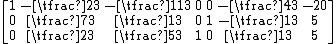
Now columns 4 and 5 represent the basic variables z and s and the corresponding basic feasible solution is
For the next step, there are no positive entries in the objective row and in fact
so the minimum value of Z is −20.
Finding an initial canonical tableau
In general, a linear program will not be given in canonical form and an equivalent canonical tableau must be found before the simplex algorithm can start. This can be accomplished by the introduction of artificial variables. Columns of the identity matrix are added as column vectors for these variables. The new tableau is in canonical form but it is not equivalent to the original problem. So a new objective function, equal to the sum of the artificial variables, is introduced and the simplex algorithm is applied to find the minimum; the modified linear program is called the Phase I problem.
The simplex algorithm applied to the Phase I problem must terminate with a minimum value for the new objective function since, being the sum of nonnegative variables, its value is bounded below by 0. If the minimum is 0 then the artificial variables can be eliminated from the resulting canonical tableau producing a canonical tableau equivalent to the original problem. The simplex algorithm can then be applied to find the solution; this step is called Phase II. If the minimum is positive then there is no feasible solution for the Phase I problem where the artificial variables are all zero. This implies that the feasible region for the original problem is empty, and so the original problem has no solution.
Example
Consider the linear program- Minimize
- Subject to

This is represented by the (non-canonical) tableau
Introduce artificial variables u and v and objective function W = u + v, giving a new tableau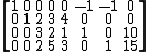
Note that the equation defining the original objective function is retained in anticipation of Phase II. After pricing out this becomes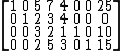
Select column 5 as a pivot column, so the pivot row must be row 4, and the updated tableau is
Now select column 3 as a pivot column, for which row 3 must be the pivot row, to get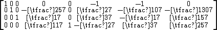
The artificial variables are now 0 and they may be dropped giving a canonical tableau equivalent to the original problem: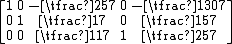
This is, fortuitously, already optimal and the optimum value for the original linear program is −130/7.
Implementation
The tableau form used above to describe the algorithm lends itself to an immediate implementation in which the tableau is maintained as a rectangular (m + 1)-by-(m + n + 1) array. It is straightforward to avoid storing the m explicit columns of the identity matrix that will occur within the tableau by virtue of B being a subset of the columns of [A, I]. This implementation is referred to as the "standard simplex algorithm". The storage and computation overhead are such that the standard simplex method is a prohibitively expensive approach to solving large linear programming problems.
In each simplex iteration, the only data required are the first row of the tableau, the (pivotal) column of the tableau corresponding to the entering variable and the right-hand-side. The latter can be updated using the pivotal column and the first row of the tableau can be updated using the (pivotal) row corresponding to the leaving variable. Both the pivotal column and pivotal row may be computed directly using the solutions of linear systems of equations involving the matrix B and a matrix-vector product using A. These observations motivate the "revised simplex algorithm", for which implementations are distinguished by their invertible representation of B.
In large linear-programming problems A is typically a sparse matrixSparse matrixIn the subfield of numerical analysis, a sparse matrix is a matrix populated primarily with zeros . The term itself was coined by Harry M. Markowitz....
and, when the resulting sparsity of B is exploited when maintaining its invertible representation, the revised simplex algorithm is a much more efficient than the standard simplex method. Commercial simplex solvers are based on the revised simplex algorithm.
Degeneracy: Stalling and cycling
If the values of all basic variables are strictly positive, then a pivot must result in an improvement in the objective value. When this is always the case no set of basic variables occurs twice and the simplex algorithm must terminate after a finite number of steps. Basic feasible solutions where at least one of the basic variables is zero are called degenerate and may result in pivots for which there is no improvement in the objective value. In this case there is no actual change in the solution but only a change in the set of basic variables. When several such pivots occur in succession, there is no improvement; in large industrial applications, degeneracy is common and such "stalling" is notable.
Worse than stalling is the possibility the same set of basic variables occurs twice, in which case, the deterministic pivoting rules of the simplex algorithm will produce an infinite loop, or "cycle". While degeneracy is the rule in practice and stalling is common, cycling is rare in practice. A discussion of an example of practical cycling occurs in Padberg. Bland's ruleBland's ruleIn mathematical optimization, Bland's rule is an algorithmic refinement of the simplex method for linear optimization....
prevents cycling and thus guarantee that the simplex algorithm always terminates. Another pivoting algorithm, the criss-cross algorithmCriss-cross algorithmIn mathematical optimization, the criss-cross algorithm denotes a family of algorithms for linear programming. Variants of the criss-cross algorithm also solve more general problems with linear inequality constraints and nonlinear objective functions; there are criss-cross algorithms for...
never cycles on linear programs.
Efficiency
The simplex method is remarkably efficient in practice and was a great improvement over earlier methods such as Fourier–Motzkin eliminationFourier–Motzkin eliminationFourier–Motzkin elimination, FME method, is a mathematical algorithm for eliminating variables from a system of linear inequalities. It can look for both real and integer solutions...
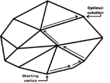
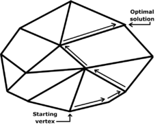
. However, in 1972, Klee and Minty gave an example showing that the worst-case complexity of simplex method as formulated by Dantzig is exponential time. Since then, for almost every variation on the method, it has been shown that there is a family of linear programs for which it performs badly. It is an open question if there is a variation with polynomial time, or even sub-exponential worst-case complexity.
Analyzing and quantifying the observation that the simplex algorithm is efficient in practice, even though it has exponential worst-case complexity, has led to the development of other measures of complexity. The simplex algorithm has polynomial-time average-case complexityBest, worst and average caseIn computer science, best, worst and average cases of a given algorithm express what the resource usage is at least, at most and on average, respectively...
under various probability distributionProbability distributionIn probability theory, a probability mass, probability density, or probability distribution is a function that describes the probability of a random variable taking certain values....
s, with the precise average-case performance of the simplex algorithm depending on the choice of a probability distribution for the random matricesRandom matrixIn probability theory and mathematical physics, a random matrix is a matrix-valued random variable. Many important properties of physical systems can be represented mathematically as matrix problems...
. Another approach to studying "typical phenomaPorous setIn mathematics, a porosity is a concept in the study of metric spaces. Like the concepts of meagre and measure zero sets, porosity is a notion of a set being somehow "sparse" or "lacking bulk"; however, porosity is not equivalent to either of the above notions, as shown below.-Definition:Let be a...
" uses Baire category theory from general topologyGeneral topologyIn mathematics, general topology or point-set topology is the branch of topology which studies properties of topological spaces and structures defined on them...
, and to show that (topologically) "most" matrices can be solved by the simplex algorithm in a polynomial number of steps. Another method to analyze the performance of the simplex algorithm studies the behavior of worst-case scenarios under small perturbation – are worst-case scenarios stable under a small change (in the sense of structural stabilityStructural stabilityIn mathematics, structural stability is a fundamental property of a dynamical system which means that the qualitative behavior of the trajectories is unaffected by C1-small perturbations....
), or do they become tractable? Formally, this method uses random problems to which is added a Gaussian random vector ("smoothed complexity").
Other algorithms
Other algorithms for solving linear-programming problems are described in the linear-programmingLinear programmingLinear programming is a mathematical method for determining a way to achieve the best outcome in a given mathematical model for some list of requirements represented as linear relationships...
article. Another basis-exchange pivoting algorithm is the criss-cross algorithmCriss-cross algorithmIn mathematical optimization, the criss-cross algorithm denotes a family of algorithms for linear programming. Variants of the criss-cross algorithm also solve more general problems with linear inequality constraints and nonlinear objective functions; there are criss-cross algorithms for...
. There are polynomial-time algorithms for linear programming that use interior point methods: These include Khachiyan's ellipsoidal algorithm, Karmarkar's projective algorithmKarmarkar's algorithmKarmarkar's algorithm is an algorithm introduced by Narendra Karmarkar in 1984 for solving linear programming problems. It was the first reasonably efficient algorithm that solves these problems in polynomial time...
, and path-following algorithmInterior point methodInterior point methods are a certain class of algorithms to solve linear and nonlinear convex optimization problems.The interior point method was invented by John von Neumann...
s.
Linear-fractional programming
Linear-fractional programmingLinear-fractional programmingIn mathematical optimization, linear-fractional programming is a generalization of linear programming . Whereas the objective function in linear programs are linear functions, the objective function in a linear-fractional program is a ratio of two linear functions...
(LFP) is a generalization of linear programmingLinear programmingLinear programming is a mathematical method for determining a way to achieve the best outcome in a given mathematical model for some list of requirements represented as linear relationships...
(LP). Where the objective function of linear programs are linear functionsLinear functionalIn linear algebra, a linear functional or linear form is a linear map from a vector space to its field of scalars. In Rn, if vectors are represented as column vectors, then linear functionals are represented as row vectors, and their action on vectors is given by the dot product, or the...
, the objective function of a linear-fractional program is a ratio of two linear functions. In other words, a linear program is a fractional-linear program in which the denominator is the constant function having the value one everywhere. A linear-fractional program can be solved by a variant of the simplex algorithm. They can be solved by the criss-cross algorithmCriss-cross algorithmIn mathematical optimization, the criss-cross algorithm denotes a family of algorithms for linear programming. Variants of the criss-cross algorithm also solve more general problems with linear inequality constraints and nonlinear objective functions; there are criss-cross algorithms for...
, also.
See also
- Criss-cross algorithmCriss-cross algorithmIn mathematical optimization, the criss-cross algorithm denotes a family of algorithms for linear programming. Variants of the criss-cross algorithm also solve more general problems with linear inequality constraints and nonlinear objective functions; there are criss-cross algorithms for...
- Fourier–Motzkin eliminationFourier–Motzkin eliminationFourier–Motzkin elimination, FME method, is a mathematical algorithm for eliminating variables from a system of linear inequalities. It can look for both real and integer solutions...
- Karmarkar's algorithmKarmarkar's algorithmKarmarkar's algorithm is an algorithm introduced by Narendra Karmarkar in 1984 for solving linear programming problems. It was the first reasonably efficient algorithm that solves these problems in polynomial time...
- Pivoting rule of Bland, which avoids cyclingBland's ruleIn mathematical optimization, Bland's rule is an algorithmic refinement of the simplex method for linear optimization....
- Nelder–Mead simplicial heuristic
Further reading
These introductions are written for students of computer scienceComputer scienceComputer science or computing science is the study of the theoretical foundations of information and computation and of practical techniques for their implementation and application in computer systems...
and operations researchOperations researchOperations research is an interdisciplinary mathematical science that focuses on the effective use of technology by organizations...
:- Thomas H. CormenThomas H. CormenThomas H. Cormen is the co-author of Introduction to Algorithms, along with Charles Leiserson, Ron Rivest, and Cliff Stein. He is a Full Professor of computer science at Dartmouth College and currently Chair of the Dartmouth College Department of Computer Science. Between 2004 and 2008 he directed...
, Charles E. LeisersonCharles E. LeisersonCharles Eric Leiserson is a computer scientist, specializing in the theory of parallel computing and distributed computing, and particularly practical applications thereof; as part of this effort, he developed the Cilk multithreaded language...
, Ronald L. Rivest, and Clifford SteinClifford SteinClifford Stein, a computer scientist, is currently a professor of industrial engineering and operations research at Columbia University in New York, NY, where he also holds an appointment in the Department of Computer Science. Stein is chair of the Industrial Engineering and Operations Research...
. Introduction to Algorithms, Second Edition. MIT Press and McGraw-Hill, 2001. ISBN 0-262-03293-7. Section 29.3: The simplex algorithm, pp. 790–804. - Frederick S. Hillier and Gerald J. Lieberman: Introduction to Operations Research, 8th edition. McGraw-Hill. ISBN 0-07-123828-X
External links
- An Introduction to Linear Programming and the Simplex Algorithm by Spyros Reveliotis of the Georgia Institute of Technology.
- Greenberg, Harvey J., Klee-Minty Polytope Shows Exponential Time Complexity of Simplex Method University of Colorado at Denver (1997) PDF download
- Simplex Method A tutorial for Simplex Method with examples (also two-phase and M-method).
- Criss-cross algorithm
- Minimize