Numerical integration
Encyclopedia
Numerical analysis
Numerical analysis is the study of algorithms that use numerical approximation for the problems of mathematical analysis ....
, numerical integration constitutes a broad family of algorithms for calculating the numerical value of a definite integral
Integral
Integration is an important concept in mathematics and, together with its inverse, differentiation, is one of the two main operations in calculus...
, and by extension, the term is also sometimes used to describe the numerical solution of differential equations
Numerical ordinary differential equations
Numerical ordinary differential equations is the part of numerical analysis which studies the numerical solution of ordinary differential equations...
. This article focuses on calculation of definite integrals. The term numerical quadrature (often abbreviated to quadrature
Quadrature (mathematics)
Quadrature — historical mathematical term which means calculating of the area. Quadrature problems have served as one of the main sources of mathematical analysis.- History :...
) is more or less a synonym for numerical integration, especially as applied to one-dimensional integrals. Numerical integration over more than one dimension is sometimes described as cubature, although the meaning of quadrature is understood for higher dimensional integration as well.
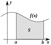
The basic problem considered by numerical integration is to compute an approximate solution to a definite integral:

If is a smooth well-behaved function, integrated over a small number of dimensions and the limits of integration are bounded, there are many methods of approximating the integral with arbitrary precision.
Reasons for numerical integration
There are several reasons for carrying out numerical integration.The integrand f(x) may be known only at certain points,
such as obtained by sampling
Sampling (statistics)
In statistics and survey methodology, sampling is concerned with the selection of a subset of individuals from within a population to estimate characteristics of the whole population....
.
Some embedded systems and other computer applications may need numerical integration for this reason.
A formula for the integrand may be known, but it may be difficult or impossible to find an antiderivative
Antiderivative
In calculus, an "anti-derivative", antiderivative, primitive integral or indefinite integralof a function f is a function F whose derivative is equal to f, i.e., F ′ = f...
which is an elementary function. An example of such an integrand is f(x) = exp(−x2), the antiderivative of which (the error function
Error function
In mathematics, the error function is a special function of sigmoid shape which occurs in probability, statistics and partial differential equations...
, times a constant) cannot be written in elementary form.
It may be possible to find an antiderivative symbolically, but it may be easier to compute a numerical approximation than to compute the antiderivative. That may be the case if the antiderivative is given as an infinite series or product, or if its evaluation requires a special function which is not available.
Methods for one-dimensional integrals
Numerical integration methods can generally be described as combining evaluations of the integrand to get an approximation to the integral. The integrand is evaluated at a finite set of points called integration points and a weighted sum of these values is used to approximate the integral. The integration points and weights depend on the specific method used and the accuracy required from the approximation.An important part of the analysis of any numerical integration method is to study the behavior of the approximation error as a function of the number of integrand evaluations.
A method which yields a small error for a small number of evaluations is usually considered superior.
Reducing the number of evaluations of the integrand reduces the number of arithmetic operations involved,
and therefore reduces the total round-off error
Round-off error
A round-off error, also called rounding error, is the difference between the calculated approximation of a number and its exact mathematical value. Numerical analysis specifically tries to estimate this error when using approximation equations and/or algorithms, especially when using finitely many...
.
Also,
each evaluation takes time, and the integrand may be arbitrarily complicated.
A 'brute force' kind of numerical integration can be done, if the integrand is reasonably well-behaved (i.e. piecewise
Piecewise
On mathematics, a piecewise-defined function is a function whose definition changes depending on the value of the independent variable...
continuous
Continuous function
In mathematics, a continuous function is a function for which, intuitively, "small" changes in the input result in "small" changes in the output. Otherwise, a function is said to be "discontinuous". A continuous function with a continuous inverse function is called "bicontinuous".Continuity of...
and of bounded variation
Bounded variation
In mathematical analysis, a function of bounded variation, also known as a BV function, is a real-valued function whose total variation is bounded : the graph of a function having this property is well behaved in a precise sense...
), by evaluating the integrand with very small increments.
Quadrature rules based on interpolating functions
A large class of quadrature rules can be derived by constructing interpolatingInterpolation
In the mathematical field of numerical analysis, interpolation is a method of constructing new data points within the range of a discrete set of known data points....
functions which are easy to integrate. Typically these interpolating functions are polynomial
Polynomial
In mathematics, a polynomial is an expression of finite length constructed from variables and constants, using only the operations of addition, subtraction, multiplication, and non-negative integer exponents...
s.
The simplest method of this type is to let the interpolating function be a constant function (a polynomial of degree zero) which passes through the point ((a+b)/2, f((a+b)/2)). This is called the midpoint rule or rectangle rule
Rectangle method
In mathematics, specifically in integral calculus, the rectangle method computes an approximation to a definite integral, made by finding the area of a collection of rectangles whose heights are determined by the values of the function.Specifically, the interval over which the function is to be...
.

The interpolating function may be an affine function (a polynomial of degree 1)
which passes through the points (a, f(a)) and (b, f(b)).
This is called the trapezoidal rule.


where the subintervals have the form [k h, (k+1) h], with h = (b−a)/n and k = 0, 1, 2, ..., n−1.
Interpolation with polynomials evaluated at equally spaced points in [a, b] yields the Newton–Cotes formulas, of which the rectangle rule and the trapezoidal rule are examples. Simpson's rule
Simpson's rule
In numerical analysis, Simpson's rule is a method for numerical integration, the numerical approximation of definite integrals. Specifically, it is the following approximation:...
, which is based on a polynomial of order 2, is also a Newton–Cotes formula.
Quadrature rules with equally spaced points have the very convenient property of nesting. The corresponding rule with each interval subdivided includes all the current points, so those integrand values can be re-used.
If we allow the intervals between interpolation points to vary, we find another group of quadrature formulas, such as the Gaussian quadrature
Gaussian quadrature
In numerical analysis, a quadrature rule is an approximation of the definite integral of a function, usually stated as a weighted sum of function values at specified points within the domain of integration....
formulas. A Gaussian quadrature rule is typically more accurate than a Newton–Cotes rule which requires the same number of function evaluations, if the integrand is smooth
Smooth function
In mathematical analysis, a differentiability class is a classification of functions according to the properties of their derivatives. Higher order differentiability classes correspond to the existence of more derivatives. Functions that have derivatives of all orders are called smooth.Most of...
(i.e., if it is sufficiently differentiable) Other quadrature methods with varying intervals include Clenshaw–Curtis quadrature (also called Fejér quadrature) methods.
Gaussian quadrature rules do not nest, but the related Gauss–Kronrod quadrature formulas do. Clenshaw–Curtis rules nest.
Adaptive algorithms
If f(x) does not have many derivatives at all points, or if the derivatives become large, then Gaussian quadrature is often insufficient. In this case, an algorithm similar to the following will perform better:def calculate_definite_integral_of_f(f, initial_step_size):
This algorithm calculates the definite integral of a function
from 0 to 1, adaptively, by choosing smaller steps near
problematic points.
x = 0.0
h = initial_step_size
accumulator = 0.0
while x < 1.0:
if x + h > 1.0:
h = 1.0 - x
quad_this_step =
if error_too_big_in_quadrature_of_over_range(f, [x,x+h]):
h = make_h_smaller(h)
else:
accumulator += quadrature_of_f_over_range(f, [x,x+h])
x += h
if error_too_small_in_quadrature_of_over_range(f, [x,x+h]):
h = make_h_larger(h) # Avoid wasting time on tiny steps.
return accumulator
Some details of the algorithm require careful thought. For many cases, estimating the error from quadrature over an interval for a function f(x) isn't obvious. One popular solution is to use two different rules of quadrature, and use their difference as an estimate of the error from quadrature. The other problem is deciding what "too large" or "very small" signify. A local criterion for "too large" is that the quadrature error should not be larger than t · h where t, a real number, is the tolerance we wish to set for global error. Then again, if h is already tiny, it may not be worthwhile to make it even smaller even if the quadrature error is apparently large. A global criterion is that the sum of errors on all the intervals should be less than t. This type of error analysis is usually called "a posteriori" since we compute the error after having computed the approximation.
Heuristics for adaptive quadrature are discussed by Forsythe et al. (Section 5.4).
Extrapolation methods
The accuracy of a quadrature rule of the Newton-Cotes type is generally a function of the number of evaluation points.The result is usually more accurate as number of evaluation points increases,
or, equivalently, as the width of the step size between the points decreases.
It is natural to ask what the result would be if the step size were allowed to approach zero.
This can be answered by extrapolating the result from two or more nonzero step sizes, using series acceleration
Series acceleration
In mathematics, series acceleration is one of a collection of sequence transformations for improving the rate of convergence of a series. Techniques for series acceleration are often applied in numerical analysis, where they are used to improve the speed of numerical integration...
methods such as Richardson extrapolation
Richardson extrapolation
In numerical analysis, Richardson extrapolation is a sequence acceleration method, used to improve the rate of convergence of a sequence. It is named after Lewis Fry Richardson, who introduced the technique in the early 20th century. In the words of Birkhoff and Rota, ".....
.
The extrapolation function may be a polynomial
Polynomial
In mathematics, a polynomial is an expression of finite length constructed from variables and constants, using only the operations of addition, subtraction, multiplication, and non-negative integer exponents...
or rational function
Rational function
In mathematics, a rational function is any function which can be written as the ratio of two polynomial functions. Neither the coefficients of the polynomials nor the values taken by the function are necessarily rational.-Definitions:...
.
Extrapolation methods are described in more detail by Stoer and Bulirsch (Section 3.4) and are implemented in many of the routines in the QUADPACK
QUADPACK
QUADPACK is a FORTRAN 77 library for numerical integration of one-dimensional functions. It was included in the SLATEC Common Mathematical Library and is therefore in the public domain. The individual subprograms are also available on netlib....
library.
Conservative (a priori) error estimation
Let f have a bounded first derivative over [a,b]. The mean value theoremMean value theorem
In calculus, the mean value theorem states, roughly, that given an arc of a differentiable curve, there is at least one point on that arc at which the derivative of the curve is equal to the "average" derivative of the arc. Briefly, a suitable infinitesimal element of the arc is parallel to the...
for f, where x < b, gives

for some yx in [a,x] depending on x. If we integrate in x from a to b on both sides and take the absolute values, we obtain
-

We can further approximate the integral on the right-hand side by bringing the absolute value into the integrand, and replacing the term in f' by an upper bound:
-
 (**)
(**)
(See supremumSupremumIn mathematics, given a subset S of a totally or partially ordered set T, the supremum of S, if it exists, is the least element of T that is greater than or equal to every element of S. Consequently, the supremum is also referred to as the least upper bound . If the supremum exists, it is unique...
.) Hence, if we approximate the integral ∫ab f(x) dx by the quadrature rule (b − a)f(a) our error is no greater than the right hand side of (**). We can convert this into an error analysis for the Riemann sum (*), giving an upper bound of
for the error term of that particular approximation. (Note that this is precisely the error we calculated for the example .) Using more derivatives, and by tweaking the quadrature, we can do a similar error analysis using a Taylor seriesTaylor seriesIn mathematics, a Taylor series is a representation of a function as an infinite sum of terms that are calculated from the values of the function's derivatives at a single point....
(using a partial sum with remainder term) for f. This error analysis gives a strict upper bound on the error, if the derivatives of f are available.
This integration method can be combined with interval arithmeticInterval arithmeticInterval arithmetic, interval mathematics, interval analysis, or interval computation, is a method developed by mathematicians since the 1950s and 1960s as an approach to putting bounds on rounding errors and measurement errors in mathematical computation and thus developing numerical methods that...
to produce computer proofs and verified calculations.
Infinite intervals
One way to calculate an integral over infinite interval,

is to transform it into an integral over a finite interval by any one of several possible changes of variables, for example:

The integral over finite interval can then be evaluated by ordinary integration methods.
Half-infinite intervals
An integral over a half-infinite interval can likewise be transformed into an integral over a finite interval by any one of several possible changes of variables, for example:

Similarly,
Multidimensional integrals
The quadrature rules discussed so far are all designed to compute one-dimensional integrals.
To compute integrals in multiple dimensions,
one approach is to phrase the multiple integral as repeated one-dimensional integrals by appealing to Fubini's theoremFubini's theoremIn mathematical analysis Fubini's theorem, named after Guido Fubini, is a result which gives conditions under which it is possible to compute a double integral using iterated integrals. As a consequence it allows the order of integration to be changed in iterated integrals.-Theorem...
.
This approach requires the function evaluations to grow exponentiallyExponential growthExponential growth occurs when the growth rate of a mathematical function is proportional to the function's current value...
as the number of dimensions increases. Two methods are known to overcome this so-called curse of dimensionalityCurse of dimensionalityThe curse of dimensionality refers to various phenomena that arise when analyzing and organizing high-dimensional spaces that do not occur in low-dimensional settings such as the physical space commonly modeled with just three dimensions.There are multiple phenomena referred to by this name in...
.
Monte Carlo
Monte Carlo methodMonte Carlo methodMonte Carlo methods are a class of computational algorithms that rely on repeated random sampling to compute their results. Monte Carlo methods are often used in computer simulations of physical and mathematical systems...
s and quasi-Monte Carlo methodQuasi-Monte Carlo methodIn numerical analysis, a quasi-Monte Carlo method is a method for the computation of an integral that is based on low-discrepancy sequences...
s are easy to apply to multi-dimensional integrals,
and may yield greater accuracy for the same number of function evaluations than repeated integrations using one-dimensional methods.
A large class of useful Monte Carlo methods are the so-called Markov chain Monte CarloMarkov chain Monte CarloMarkov chain Monte Carlo methods are a class of algorithms for sampling from probability distributions based on constructing a Markov chain that has the desired distribution as its equilibrium distribution. The state of the chain after a large number of steps is then used as a sample of the...
algorithms,
which include the Metropolis-Hastings algorithmMetropolis-Hastings algorithmIn mathematics and physics, the Metropolis–Hastings algorithm is a Markov chain Monte Carlo method for obtaining a sequence of random samples from a probability distribution for which direct sampling is difficult...
and Gibbs samplingGibbs samplingIn statistics and in statistical physics, Gibbs sampling or a Gibbs sampler is an algorithm to generate a sequence of samples from the joint probability distribution of two or more random variables...
.
Sparse grids
Sparse gridSparse gridSparse grids are numerical techniques to represent, integrate or interpolate high dimensional functions. They were originally found by the Russian mathematician Smolyak and are based on a sparse tensor product construction...
s were originally developed by Smolyak for the quadrature of high dimensional functions. The method is always based on a one dimensional quadrature rule, but performs a more sophisticated combination of univariate results.
Connection with differential equations
The problem of evaluating the integral
can be reduced to an initial value problemInitial value problemIn mathematics, in the field of differential equations, an initial value problem is an ordinary differential equation together with a specified value, called the initial condition, of the unknown function at a given point in the domain of the solution...
for an ordinary differential equationOrdinary differential equationIn mathematics, an ordinary differential equation is a relation that contains functions of only one independent variable, and one or more of their derivatives with respect to that variable....
. If the above integral is denoted by I(b), then the function I satisfies
Methods developed for ordinary differential equations, such as Runge–Kutta methodsRunge–Kutta methodsIn numerical analysis, the Runge–Kutta methods are an important family of implicit and explicit iterative methods for the approximation of solutions of ordinary differential equations. These techniques were developed around 1900 by the German mathematicians C. Runge and M.W. Kutta.See the article...
, can be applied to the restated problem and thus be used to evaluate the integral. For instance, the standard fourth-order Runge–Kutta method applied to the differential equation yields Simpson's rule from above.
The differential equation I ' (x) = ƒ(x) has a special form: the right-hand side contains only the dependent variable (here x) and not the independent variable (here I). This simplifies the theory and algorithms considerably. The problem of evaluating integrals is thus best studied in its own right.
See also
- Numerical ordinary differential equationsNumerical ordinary differential equationsNumerical ordinary differential equations is the part of numerical analysis which studies the numerical solution of ordinary differential equations...
- Truncation error (numerical integration)Truncation error (numerical integration)Trunction errors in numerical integration are of two kinds:* local truncation errors – the error caused by one iteration, and* global truncation errors – the cumulative error cause by many iterations.- Definitions :...
External links
- Integration: Background, Simulations, etc. at Holistic Numerical Methods Institute
Free software for numerical integration
Numerical integration is one of the most intensively studied problems in numerical analysis.
Of the many software implementations, we list a few free and open source softwareFree and open source softwareFree and open-source software or free/libre/open-source software is software that is liberally licensed to grant users the right to use, study, change, and improve its design through the availability of its source code...
packages here:
- QUADPACKQUADPACKQUADPACK is a FORTRAN 77 library for numerical integration of one-dimensional functions. It was included in the SLATEC Common Mathematical Library and is therefore in the public domain. The individual subprograms are also available on netlib....
(part of SLATEC): description http://www.netlib.org/slatec/src/qpdoc.f, source code http://www.netlib.org/slatec/src. QUADPACK is a collection of algorithms, in Fortran, for numerical integration based on Gaussian quadrature. - interalg: a solver from OpenOptOpenOptOpenOpt is an open-source framework for numerical optimization, nonlinear equations and systems of them. It is licensed under the BSD license, making it available to be used in both open- and closed-code software. The package already has some essential ....
/FuncDesignerFuncDesignerFuncDesigner is a computer algebra system written as a Python module. It is cross-platform software , with a completely free license....
frameworks, based on interval analysis, guaranteed precision, license: BSD (free for any purposes) - GSL: The GNU Scientific Library (GSL) is a numerical library written in C which provides a wide range of mathematical routines, like Monte Carlo integration.
- Numerical integration algorithms are found in GAMSGuide to Available Mathematical SoftwareThe Guide to Available Mathematical Software is a project of the National Institute of Standards and Technology to classify mathematical software by the type of problem that it solves. GAMS indexes Netlib, and also some proprietary software packages....
class H2. - ALGLIB is a collection of algorithms, in C# / C++ / Delphi / Visual Basic / etc., for numerical integration (includes Bulirsch-Stoer and Runge-Kutta integrators).
- Cuba is a free-software library of several multi-dimensional integration algorithms.
- Cubature code for adaptive multi-dimensional integration.
- Cubature formulas for the 2D unit disk Derivation, source code for product-type Gaussian cubature with high precision coefficients and nodes.
- High-precision abscissas and weights for Gaussian Quadrature for n = 2, ..., 20, 32, 64, 100, 128, 256, 512, 1024 also contains C language source code under LGPL license.
-