The polar method is a pseudo-random number sampling

Pseudo-random number sampling

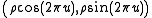
Pseudo-random number sampling or non-uniform pseudo-random variate generation is the numerical practice of generating pseudo-random numbers that are distributed according to a given probability distribution....

 method for generating a pair of independent standard normal random variables. While it is superior to the Box–Muller transform, the Ziggurat algorithm

Ziggurat algorithm

The ziggurat algorithm is an algorithm for pseudo-random number sampling. Belonging to the class of rejection sampling algorithms, it relies on an underlying source of uniformly-distributed random numbers, typically from a pseudo-random number generator, as well as precomputed tables. The...

 is even more efficient.

Standard normal random variables are frequently used in computer science

Computer science

Computer science or computing science is the study of the theoretical foundations of information and computation and of practical techniques for their implementation and application in computer systems...

, computational statistics

Computational statistics

Computational statistics, or statistical computing, is the interface between statistics and computer science. It is the area of computational science specific to the mathematical science of statistics....

, and in particular, in applications of the Monte Carlo method

Monte Carlo method

Monte Carlo methods are a class of computational algorithms that rely on repeated random sampling to compute their results. Monte Carlo methods are often used in computer simulations of physical and mathematical systems...

.

The polar method works by choosing random points (x, y) in the square −1 < x < 1, −1 < y < 1 until


and then returning the required pair of normal random variables as

Theoretical basis

The underlying theory may be summarized as follows:

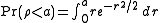
If u is uniformly distributed in the interval
0 ≤ u < 1, then the point
(cos(2πu), sin(2πu))
is uniformly distributed on the unit circumference
x² + y² = 1, and multiplying that point by an independent
random variable ρ whose distribution is


will produce a point


whose coordinates are jointly distributed as two independent standard
normal random variables.

History

This idea dates back to Laplace, whom Gauss credits with finding the above


by taking the square root of


The transformation to polar coordinates makes evident that θ is
uniformly distributed (constant density) from 0 to 2π, and that the
radial distance r has density


(Note that r² has the appropriate chi square distribution.)

This method of producing a pair of independent standard normal variates by radially projecting a random point on the unit circumference to a distance given by the square root of a chi-square-2 variate is called the polar method for generating a pair of normal random variables,

Practical considerations

A direct application of this idea,


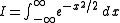
is called the Box Muller transform, in which the chi variate is usually
generated as


but that transform requires logarithm, square root, sine and cosine functions. On some processors, the cosine and sine of the same argument can be calculated in parallel using a single instruction. Notably for Intel based machines, one can use fsincos assembler instruction or the expi instruction (available i.e. in D), to calculate complex

and just separate the real and imaginary parts.

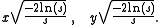
The polar method, in which
a random point (x, y) inside the unit circle
is projected onto the unit circumference by setting s = x² + y² and forming the point


is a faster procedure. Some researchers argue that the conditional if instruction (for rejecting a point outside of the unit circle), can make programs slower on modern processors equipped with pipelining and branch prediction. Also this procedure requires about 27% more evaluations of the underlying random number generator (only of generated points lie inside of unit circle).

That random point on the circumference is then radially projected the required random distance by means of


using the same s because that s is independent of the random point on the circumference and is itself uniformly distributed from 0 to 1.

Implementation

Simple implementation in java;

private static double spare;
private static boolean spareready = false;

public static synchronized double getGaussian(double center, double stdDev) {
if (spareready) {
spareready = false;
return spare * stdDev + center;
}
double u, v, s;
do {
u = Math.random * 2 - 1;
v = Math.random * 2 - 1;
s = u * u + v * v;
} while (s >= 1 || s 0);
spare = v * Math.sqrt(-2 * Math.log(s) / s);
spareready = true;
return center + stdDev * u * Math.sqrt(-2.0 * Math.log(s) / s);
}