

Marcinkiewicz theorem
Encyclopedia
In mathematics
, the Marcinkiewicz interpolation theorem, discovered by , is a result bounding the norms of non-linear operators acting on Lp spaces
.
Marcinkiewicz' theorem is similar to the Riesz–Thorin theorem about linear operators, but also applies to non-linear operators.
with real or complex values, defined on a measure space (X, F, ω). The distribution function
of f is defined by

Then f is called weak if there exists a constant C such that the distribution of f satisfies the following inequality for all t > 0:

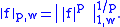
The smallest constant C in the inequality above is called the weak norm and is usually denoted by ||f||1,w or ||f||1,∞. Similarly the space is usually denoted by L1,w or L1,∞.
(Note: This terminology is a bit misleading since the weak norm does not satisfy the triangle inequality as one can see by considering the sum of the functions on given by
  and
and  , which has norm 4 not 2.)
Any function belongs to L1,w and in addition one has the inequality

This is nothing but Markov's inequality
. The converse is not true. For example, the function 1/x belongs to L1,w but not to L1.
Similarly, one may define the weak space as the space of all functions f such that
  belong to L1,w, and the weak
  norm using
More directly, the Lp,w norm is defined as the best constant C in the inequality

for all t > 0.
Theorem: Let T be a bounded linear operator from to
to  and at the same time from
  to
to  . Then T is also a bounded operator from
  to
to  for any r between p and q.
In other words, even if you only require weak boundedness on the extremes p and q, you still get regular boundedness inside. To make this more formal, one has to explain that T is bounded only on a dense subset and can be completed. See Riesz-Thorin theorem
for these details.
Where Marcinkiewicz's theorem is weaker than the Riesz-Thorin theorem is in the estimates of the norm. The theorem gives bounds for the norm of T but this bound increases to infinity as r converges to either p or q. Specifically , suppose that
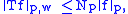

so that the operator norm
of T from Lp to Lp,w is at most Np, and the operator norm of T from Lq to Lq,w is at most Nq. Then the following interpolation inequality holds for all r between p and q and all f ∈ Lr: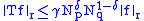
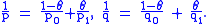
where
and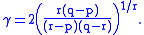
The constants δ and γ can also be given for q = ∞ by passing to the limit.
A version of the theorem also holds more generally if T is only assumed to be a quasilinear
operator. That is, there exists a constant C > 0 such that T satisfies
for almost every
x. The theorem holds precisely as stated, except with γ replaced by
An operator T (possibly quasilinear) satisfying an estimate of the form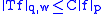
is said to be of weak type (p,q). An operator is simply of type (p,q) if T is a bounded transformation from Lp to Lq:
A more general formulation of the interpolation theorem is as follows:
The latter formulation follows from the former through an application of Hölder's inequality
and a duality argument.
. Viewed as a multiplier
, the Hilbert transform of a function f can be computed by first taking the Fourier transform
of f, then multiplying by the sign function
, and finally applying the inverse Fourier transform.
Hence Parseval's theorem
easily shows that the Hilbert transform is bounded from to
to  . A much less obvious fact is that it is bounded from
  to
to  . Hence Marcinkiewicz's theorem shows that it is bounded from
  to
to  for any 1 < p < 2. Duality
arguments show that it is also bounded for 2 < p < ∞. In fact, the Hilbert transform is really unbounded for p equal to 1 or ∞.
Another famous example is the Hardy–Littlewood maximal function, which is only quasilinear rather than linear. While to
to  bounds can be derived immediately from the
  to weak
  estimate by a clever change of variables, Marcinkiewicz interpolation is a more intuitive approach. Since the Hardy–Littlewood Maximal Function is trivially bounded from
  to
to  , strong boundedness for all
  follows immediately from the weak (1,1) estimate and interpolation.
shortly before he died in World War II. The theorem was almost forgotten by Zygmund, and was absent from his original works on the theory of singular integral operators. Later realized that Marcinkiewicz's result could greatly simplify his work, at which time he published his former student's theorem together with a generalization of his own.
Mathematics
Mathematics is the study of quantity, space, structure, and change. Mathematicians seek out patterns and formulate new conjectures. Mathematicians resolve the truth or falsity of conjectures by mathematical proofs, which are arguments sufficient to convince other mathematicians of their validity...
, the Marcinkiewicz interpolation theorem, discovered by , is a result bounding the norms of non-linear operators acting on Lp spaces
Lp space
In mathematics, the Lp spaces are function spaces defined using a natural generalization of the p-norm for finite-dimensional vector spaces...
.
Marcinkiewicz' theorem is similar to the Riesz–Thorin theorem about linear operators, but also applies to non-linear operators.
Preliminaries
Let f be a measurable functionMeasurable function
In mathematics, particularly in measure theory, measurable functions are structure-preserving functions between measurable spaces; as such, they form a natural context for the theory of integration...
with real or complex values, defined on a measure space (X, F, ω). The distribution function
Cumulative distribution function
In probability theory and statistics, the cumulative distribution function , or just distribution function, describes the probability that a real-valued random variable X with a given probability distribution will be found at a value less than or equal to x. Intuitively, it is the "area so far"...
of f is defined by
Then f is called weak
if there exists a constant C such that the distribution of f satisfies the following inequality for all t > 0:The smallest constant C in the inequality above is called the weak
norm and is usually denoted by ||f||1,w or ||f||1,∞. Similarly the space is usually denoted by L1,w or L1,∞.(Note: This terminology is a bit misleading since the weak norm does not satisfy the triangle inequality as one can see by considering the sum of the functions on
given by and , which has norm 4 not 2.)Any
function belongs to L1,w and in addition one has the inequalityThis is nothing but Markov's inequality
Markov's inequality
In probability theory, Markov's inequality gives an upper bound for the probability that a non-negative function of a random variable is greater than or equal to some positive constant...
. The converse is not true. For example, the function 1/x belongs to L1,w but not to L1.
Similarly, one may define the weak
space as the space of all functions f such that belong to L1,w, and the weak norm usingMore directly, the Lp,w norm is defined as the best constant C in the inequality
for all t > 0.
Formulation
Informally, Marcinkiewicz's theorem isTheorem: Let T be a bounded linear operator from
to and at the same time from to . Then T is also a bounded operator from to for any r between p and q.In other words, even if you only require weak boundedness on the extremes p and q, you still get regular boundedness inside. To make this more formal, one has to explain that T is bounded only on a dense subset and can be completed. See Riesz-Thorin theorem
Riesz-Thorin theorem
In mathematics, the Riesz–Thorin theorem, often referred to as the Riesz–Thorin interpolation theorem or the Riesz–Thorin convexity theorem is a result about interpolation of operators. It is named after Marcel Riesz and his student G. Olof Thorin.This theorem bounds the norms of linear maps...
for these details.
Where Marcinkiewicz's theorem is weaker than the Riesz-Thorin theorem is in the estimates of the norm. The theorem gives bounds for the
norm of T but this bound increases to infinity as r converges to either p or q. Specifically , suppose thatso that the operator norm
Operator norm
In mathematics, the operator norm is a means to measure the "size" of certain linear operators. Formally, it is a norm defined on the space of bounded linear operators between two given normed vector spaces.- Introduction and definition :...
of T from Lp to Lp,w is at most Np, and the operator norm of T from Lq to Lq,w is at most Nq. Then the following interpolation inequality holds for all r between p and q and all f ∈ Lr:
where
and
The constants δ and γ can also be given for q = ∞ by passing to the limit.
A version of the theorem also holds more generally if T is only assumed to be a quasilinear
Quasilinear
Quasilinear may refer to:* Quasilinear function, a function that is both quasiconvex and quasiconcave* Quasilinear utility, an economic utility function linear in one argument...
operator. That is, there exists a constant C > 0 such that T satisfies
for almost every
Almost everywhere
In measure theory , a property holds almost everywhere if the set of elements for which the property does not hold is a null set, that is, a set of measure zero . In cases where the measure is not complete, it is sufficient that the set is contained within a set of measure zero...
x. The theorem holds precisely as stated, except with γ replaced by
An operator T (possibly quasilinear) satisfying an estimate of the form
is said to be of weak type (p,q). An operator is simply of type (p,q) if T is a bounded transformation from Lp to Lq:
A more general formulation of the interpolation theorem is as follows:
- If T is a quasilinear operator of weak type (p0, q0) and of weak type (p1, q1) where q0 ≠ q1, then for each θ ∈ (0,1), T is of type (p,q), for p and q with p ≤ q of the form
The latter formulation follows from the former through an application of Hölder's inequality
Hölder's inequality
In mathematical analysis Hölder's inequality, named after Otto Hölder, is a fundamental inequality between integrals and an indispensable tool for the study of Lp spaces....
and a duality argument.
Applications and examples
A famous application example is the Hilbert transformHilbert transform
In mathematics and in signal processing, the Hilbert transform is a linear operator which takes a function, u, and produces a function, H, with the same domain. The Hilbert transform is named after David Hilbert, who first introduced the operator in order to solve a special case of the...
. Viewed as a multiplier
Multiplier (Fourier analysis)
In Fourier analysis, a multiplier operator is a type of linear operator, or transformation of functions. These operators act on a function by altering its Fourier transform. Specifically they multiply the Fourier transform of a function by a specified function known as the multiplier or symbol...
, the Hilbert transform of a function f can be computed by first taking the Fourier transform
Fourier transform
In mathematics, Fourier analysis is a subject area which grew from the study of Fourier series. The subject began with the study of the way general functions may be represented by sums of simpler trigonometric functions...
of f, then multiplying by the sign function
Sign function
In mathematics, the sign function is an odd mathematical function that extracts the sign of a real number. To avoid confusion with the sine function, this function is often called the signum function ....
, and finally applying the inverse Fourier transform.
Hence Parseval's theorem
Parseval's theorem
In mathematics, Parseval's theorem usually refers to the result that the Fourier transform is unitary; loosely, that the sum of the square of a function is equal to the sum of the square of its transform. It originates from a 1799 theorem about series by Marc-Antoine Parseval, which was later...
easily shows that the Hilbert transform is bounded from
to . A much less obvious fact is that it is bounded from to . Hence Marcinkiewicz's theorem shows that it is bounded from to for any 1 < p < 2. DualityDual space
In mathematics, any vector space, V, has a corresponding dual vector space consisting of all linear functionals on V. Dual vector spaces defined on finite-dimensional vector spaces can be used for defining tensors which are studied in tensor algebra...
arguments show that it is also bounded for 2 < p < ∞. In fact, the Hilbert transform is really unbounded for p equal to 1 or ∞.
Another famous example is the Hardy–Littlewood maximal function, which is only quasilinear rather than linear. While
to bounds can be derived immediately from the to weak estimate by a clever change of variables, Marcinkiewicz interpolation is a more intuitive approach. Since the Hardy–Littlewood Maximal Function is trivially bounded from to , strong boundedness for all follows immediately from the weak (1,1) estimate and interpolation.History
The theorem was first announced by , who showed this result to Antoni ZygmundAntoni Zygmund
Antoni Zygmund was a Polish-born American mathematician.-Life:Born in Warsaw, Zygmund obtained his PhD from Warsaw University and became a professor at Stefan Batory University at Wilno...
shortly before he died in World War II. The theorem was almost forgotten by Zygmund, and was absent from his original works on the theory of singular integral operators. Later realized that Marcinkiewicz's result could greatly simplify his work, at which time he published his former student's theorem together with a generalization of his own.