
Local hidden variable theory
Encyclopedia
In quantum mechanics
, a local hidden variable theory
is one in which distant events are assumed to have no instantaneous (or at least faster-than-light
) effect on local ones.
According to the quantum entanglement
theory of quantum mechanics, on the other hand, distant events may under some circumstances have instantaneous correlations with local ones. As a result of this it is now generally accepted that there can be no interpretations of quantum mechanics which use local hidden variables. The term is most often used in discussions of the EPR paradox
and Bell's inequalities
. It is effectively synonymous with the concept of local realism, which can only correctly be applied to classical physics and not to quantum mechanics.
that the probability of a coincidence can be written in factorised form:
where is the probability of detection of particle
  with hidden variable
  by detector
  , set in direction
  , and similarly
  is the probability at detector
  , set in direction
  , for particle
  , sharing the same value of
  . The source is assumed to produce particles in the state
  with probability
  .
.
Using (1), various Bell inequalities can be derived, giving restrictions on the possible behaviour of local hidden variable models.
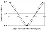
When John Bell
originally derived his inequality, it was in relation to pairs of indivisible "spin-1/2" particles, every one of those emitted being detected. In these circumstances it is found that local realist assumptions lead to a straight line prediction for the relationship between quantum correlation
and the angle between the settings of the two detectors. It was soon realised, however, that real experiments were not feasible with spin-1/2 particles. They were conducted instead using photons. The local hidden variable prediction for these is not a straight line but a sine curve, similar to the quantum mechanical prediction but of only half the "visibility".
The difference between the two predictions is due to the different functions and
and  involved. By assuming different functions, a great variety of other realist predictions can be derived, some very close to the quantum-mechanical one. The choice of function, however, is not arbitrary. In optical experiments using polarisation, for instance, the natural assumption is that it is a cosine-squared function, corresponding to adherence to Malus' Law.
Bell's theorem assumes that measurements are made at random, and not in principle determined by the universe at large. If this assumption were to be incorrect, as proposed in superdeterminism
, conclusions drawn from Bell's theorem may be invalidated. Such arguments are generally called loophole theories.
's thought-experiment (Bohm, 1951), in which a molecule breaks into two atoms with opposite spins. Assume this spin can be represented by a real vector, pointing in any direction. It will be the "hidden variable" in our model. Taking it to be a unit vector, all possible values of the hidden variable are represented by all points on the surface of a unit sphere.
Suppose the spin is to be measured in the direction a. Then the natural assumption, given that all atoms are detected, is that all atoms the projection of whose spin in the direction a is positive will be detected as spin up (coded as +1) while all whose projection is negative will be detected as spin down (coded as −1). The surface of the sphere will be divided into two regions, one for +1, one for −1, separated by a great circle
in the plane perpendicular to a. Assuming for convenience that a is horizontal, corresponding to the angle a with respect to some suitable reference direction, the dividing circle will be in a vertical plane. So far we have modelled side A of our experiment.
Now to model side B. Assume that b too is horizontal, corresponding to the angle b. There will be second great circle drawn on the same sphere, to one side of which we have +1, the other −1 for particle B. The circle will be again be in a vertical plane.
The two circles divide the surface of the sphere into four regions. The type of "coincidence" (++, −−, +− or −+) observed for any given pair of particles is determined by the region within which their hidden variable falls. Assuming the source to be "rotationally invariant" (to produce all possible states λ with equal probability), the probability of a given type of coincidence will clearly be proportional to the corresponding area, and these areas will vary linearly with the angle between a and b. (To see this, think of an orange and its segments. The area of peel corresponding to a number n of segments is roughly proportional to n. More accurately, it is proportional to the angle subtended at the centre.)
The formula (1) above has not been used explicitly — it is hardly relevant when, as here, the situation is fully deterministic. The problem could be reformulated in terms of the functions in the formula, with ρ constant and the probability functions step functions. The principle behind (1) has in fact been used, but purely intuitively.
Thus the local hidden variable prediction for the probability of coincidence is proportional to the angle (b − a) between the detector settings. The quantum correlation is defined to be the expectation value of the product of the individual outcomes, and this is
where P++ is the probability of a '+' outcome on both sides, P+− that of a + on side A, a '−' on side B, etc..
Since each individual term varies linearly with the difference (b − a), so does their sum.
The result is shown in fig. 1.
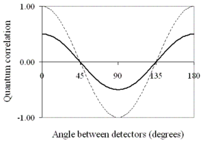
In this stochastic model, in contrast to the above deterministic case, we do need equation (1) to find the local realist prediction for coincidences. It is necessary first to make some assumption regarding the functions and
and  , the usual one being that these are both cosine-squares, in line with Malus' Law. Assuming the hidden variable to be polarisation direction (parallel on the two sides in real applications, not orthogonal), equation (1) becomes:
The predicted quantum correlation can be derived from this and is shown in fig. 2.
 In optical tests, incidentally, it is not certain that the quantum correlation is well-defined. Under a classical model of light, a single photon can go partly into the + channel, partly into the − one, resulting in the possibility of simultaneous detections in both. Though experiments such as Grangier et al.'s (Grangier, 1986) have shown that this probability is very low, it is not logical to assume that it is actually zero. The definition of quantum correlation is adapted to the idea that outcomes will always be +1, −1 or 0. There is no obvious way of including any other possibility, which is one of the reasons why Clauser and Horne's 1974 Bell test, using single-channel polarisers, should be used instead of the CHSH Bell test. The CH74 inequality concerns just probabilities of detection, not quantum correlations.
Another hypothesis suggests to review the notion of physical time (Kurakin, 2004). Hidden variables in this concept evolve in so called 'hidden time', not equivalent to physical time. Physical time relates to 'hidden time' by some 'sewing procedure'. This model stays physically non-local, though the locality is achieved in mathematical sense.
We might perhaps suppose the polarisers to be perfect, with output intensity of polariser A proportional to cos2(a − λ), but reject the quantum-mechanical assumption that the function relating this intensity to the probability of detection is a straight line through the origin. Real detectors, after all, have "dark counts" that are there even when the input intensity is zero, and become saturated when the intensity is very high. It is not possible for them to produce outputs in exact proportion to input intensity for all intensities.
By varying our assumptions, it seems possible that the realist prediction could approach the quantum-mechanical one within the limits of experimental error (Marshall, 1983), though clearly a compromise must be reached. We have to match both the behaviour of the individual light beam on passage through a polariser and the observed coincidence curves. The former would be expected to follow Malus' Law fairly closely, though experimental evidence here is not so easy to obtain. We are interested in the behaviour of very weak light and the law may be slightly different from that of stronger light.
Quantum mechanics
Quantum mechanics, also known as quantum physics or quantum theory, is a branch of physics providing a mathematical description of much of the dual particle-like and wave-like behavior and interactions of energy and matter. It departs from classical mechanics primarily at the atomic and subatomic...
, a local hidden variable theory
Hidden variable theory
Historically, in physics, hidden variable theories were espoused by some physicists who argued that quantum mechanics is incomplete. These theories argue against the orthodox interpretation of quantum mechanics, which is the Copenhagen Interpretation...
is one in which distant events are assumed to have no instantaneous (or at least faster-than-light
Faster-than-light
Faster-than-light communications and travel refer to the propagation of information or matter faster than the speed of light....
) effect on local ones.
According to the quantum entanglement
Quantum entanglement
Quantum entanglement occurs when electrons, molecules even as large as "buckyballs", photons, etc., interact physically and then become separated; the type of interaction is such that each resulting member of a pair is properly described by the same quantum mechanical description , which is...
theory of quantum mechanics, on the other hand, distant events may under some circumstances have instantaneous correlations with local ones. As a result of this it is now generally accepted that there can be no interpretations of quantum mechanics which use local hidden variables. The term is most often used in discussions of the EPR paradox
EPR paradox
The EPR paradox is a topic in quantum physics and the philosophy of science concerning the measurement and description of microscopic systems by the methods of quantum physics...
and Bell's inequalities
Bell's theorem
In theoretical physics, Bell's theorem is a no-go theorem, loosely stating that:The theorem has great importance for physics and the philosophy of science, as it implies that quantum physics must necessarily violate either the principle of locality or counterfactual definiteness...
. It is effectively synonymous with the concept of local realism, which can only correctly be applied to classical physics and not to quantum mechanics.
Local hidden variables and the Bell tests
The principle of "locality" enables the assumption to be made in Bell test experimentsBell test experiments
The Bell test experiments serve to investigate the validity of the entanglement effect in quantum mechanics by using some kind of Bell inequality...
that the probability of a coincidence can be written in factorised form:
-
- (1)

- (1)
where
is the probability of detection of particle with hidden variable by detector , set in direction , and similarly is the probability at detector , set in direction , for particle , sharing the same value of . The source is assumed to produce particles in the state with probability .Using (1), various Bell inequalities can be derived, giving restrictions on the possible behaviour of local hidden variable models.
When John Bell
John Stewart Bell
John Stewart Bell FRS was a British physicist from Northern Ireland , and the originator of Bell's theorem, a significant theorem in quantum physics regarding hidden variable theories.- Early life and work :...
originally derived his inequality, it was in relation to pairs of indivisible "spin-1/2" particles, every one of those emitted being detected. In these circumstances it is found that local realist assumptions lead to a straight line prediction for the relationship between quantum correlation
Quantum correlation
In Bell test experiments the term quantum correlation has come to mean the expectation value of the product of the outcomes on the two sides. In other words, the expected change in physical characteristics as one quantum system passes through an interaction site...
and the angle between the settings of the two detectors. It was soon realised, however, that real experiments were not feasible with spin-1/2 particles. They were conducted instead using photons. The local hidden variable prediction for these is not a straight line but a sine curve, similar to the quantum mechanical prediction but of only half the "visibility".
The difference between the two predictions is due to the different functions
and involved. By assuming different functions, a great variety of other realist predictions can be derived, some very close to the quantum-mechanical one. The choice of function, however, is not arbitrary. In optical experiments using polarisation, for instance, the natural assumption is that it is a cosine-squared function, corresponding to adherence to Malus' Law.Bell's theorem assumes that measurements are made at random, and not in principle determined by the universe at large. If this assumption were to be incorrect, as proposed in superdeterminism
Superdeterminism
In the context of quantum mechanics, superdeterminism is a term that has been used to describe a hypothetical class of theories which evade Bell's theorem by virtue of being completely deterministic. Bell's theorem depends on the assumption of counterfactual definiteness, which technically does...
, conclusions drawn from Bell's theorem may be invalidated. Such arguments are generally called loophole theories.
Bell tests with no "non-detections"
Consider, for example, David BohmDavid Bohm
David Joseph Bohm FRS was an American-born British quantum physicist who contributed to theoretical physics, philosophy, neuropsychology, and the Manhattan Project.-Youth and college:...
's thought-experiment (Bohm, 1951), in which a molecule breaks into two atoms with opposite spins. Assume this spin can be represented by a real vector, pointing in any direction. It will be the "hidden variable" in our model. Taking it to be a unit vector, all possible values of the hidden variable are represented by all points on the surface of a unit sphere.
Suppose the spin is to be measured in the direction a. Then the natural assumption, given that all atoms are detected, is that all atoms the projection of whose spin in the direction a is positive will be detected as spin up (coded as +1) while all whose projection is negative will be detected as spin down (coded as −1). The surface of the sphere will be divided into two regions, one for +1, one for −1, separated by a great circle
Great circle
A great circle, also known as a Riemannian circle, of a sphere is the intersection of the sphere and a plane which passes through the center point of the sphere, as opposed to a general circle of a sphere where the plane is not required to pass through the center...
in the plane perpendicular to a. Assuming for convenience that a is horizontal, corresponding to the angle a with respect to some suitable reference direction, the dividing circle will be in a vertical plane. So far we have modelled side A of our experiment.
Now to model side B. Assume that b too is horizontal, corresponding to the angle b. There will be second great circle drawn on the same sphere, to one side of which we have +1, the other −1 for particle B. The circle will be again be in a vertical plane.
The two circles divide the surface of the sphere into four regions. The type of "coincidence" (++, −−, +− or −+) observed for any given pair of particles is determined by the region within which their hidden variable falls. Assuming the source to be "rotationally invariant" (to produce all possible states λ with equal probability), the probability of a given type of coincidence will clearly be proportional to the corresponding area, and these areas will vary linearly with the angle between a and b. (To see this, think of an orange and its segments. The area of peel corresponding to a number n of segments is roughly proportional to n. More accurately, it is proportional to the angle subtended at the centre.)
The formula (1) above has not been used explicitly — it is hardly relevant when, as here, the situation is fully deterministic. The problem could be reformulated in terms of the functions in the formula, with ρ constant and the probability functions step functions. The principle behind (1) has in fact been used, but purely intuitively.
Thus the local hidden variable prediction for the probability of coincidence is proportional to the angle (b − a) between the detector settings. The quantum correlation is defined to be the expectation value of the product of the individual outcomes, and this is
-
- (2) E = P++ + P−− − P+− − P−+
where P++ is the probability of a '+' outcome on both sides, P+− that of a + on side A, a '−' on side B, etc..
Since each individual term varies linearly with the difference (b − a), so does their sum.
The result is shown in fig. 1.
Optical Bell tests
In almost all real applications of Bell's inequalities, the particles used have been photons. It is not necessarily assumed that the photons are particle-like. They may be just short pulses of classical light (Clauser, 1978). It is not assumed that every single one is detected. Instead the hidden variable set at the source is taken to determine only the probability of a given outcome, the actual individual outcomes being partly determined by other hidden variables local to the analyser and detector. It is assumed that these other hidden variables are independent on the two sides of the experiment (Clauser, 1974; Bell, 1971).In this stochastic model, in contrast to the above deterministic case, we do need equation (1) to find the local realist prediction for coincidences. It is necessary first to make some assumption regarding the functions
and , the usual one being that these are both cosine-squares, in line with Malus' Law. Assuming the hidden variable to be polarisation direction (parallel on the two sides in real applications, not orthogonal), equation (1) becomes:-
- (3)
 , where
  .
.
- (3)
The predicted quantum correlation can be derived from this and is shown in fig. 2.
Generalizations of the models
By varying the assumed probability and density functions in equation (1) we can arrive at a considerable variety of local realist predictions.Time effects
Previously some new hypotheses were conjectured concerning the role of time in constructing hidden variables theory. One approach is suggested by K. Hess and W. Philipp (Hess, 2002) and discusses possible consequences of time dependences of hidden variables, previously not taken into account by Bell's theorem. This hypothesis has been criticized by R.D. Gill, G. Weihs, A. Zeilinger and M. Żukowski (Gill, 2002).Another hypothesis suggests to review the notion of physical time (Kurakin, 2004). Hidden variables in this concept evolve in so called 'hidden time', not equivalent to physical time. Physical time relates to 'hidden time' by some 'sewing procedure'. This model stays physically non-local, though the locality is achieved in mathematical sense.
Optical models deviating from Malus' Law
If we make realistic (wave-based) assumptions regarding the behaviour of light on encountering polarisers and photodetectors, we find that we are not compelled to accept that the probability of detection will reflect Malus' Law exactly.We might perhaps suppose the polarisers to be perfect, with output intensity of polariser A proportional to cos2(a − λ), but reject the quantum-mechanical assumption that the function relating this intensity to the probability of detection is a straight line through the origin. Real detectors, after all, have "dark counts" that are there even when the input intensity is zero, and become saturated when the intensity is very high. It is not possible for them to produce outputs in exact proportion to input intensity for all intensities.
By varying our assumptions, it seems possible that the realist prediction could approach the quantum-mechanical one within the limits of experimental error (Marshall, 1983), though clearly a compromise must be reached. We have to match both the behaviour of the individual light beam on passage through a polariser and the observed coincidence curves. The former would be expected to follow Malus' Law fairly closely, though experimental evidence here is not so easy to obtain. We are interested in the behaviour of very weak light and the law may be slightly different from that of stronger light.