

Gaussian quadrature
Encyclopedia
In numerical analysis
, a quadrature rule is an approximation of the definite integral
of a function
, usually stated as a weighted sum of function values at specified points within the domain of integration.
(See numerical integration
for more on quadrature
rules.)
An n-point Gaussian quadrature rule, named after Carl Friedrich Gauss
, is a quadrature rule constructed to yield an exact result for polynomial
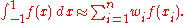
s of degree 2n − 1 or less by a suitable choice of the points xi and weights wi for i = 1,...,n.
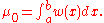
The domain of integration for such a rule is conventionally taken as [−1, 1],
so the rule is stated as
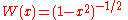
Gaussian quadrature as above will only produce accurate results if the function f(x) is well approximated by a polynomial function within the range [-1,1]. The method is not, for example, suitable for functions with singularities. However, if the integrated function can be written as
 ,
,
where g(x) is approximately polynomial, and W(x) is known, then there are alternative weights such that

Common weighting functions include
(Gauss-Chebyshev) and (Gauss-Hermite).
It can be shown (see Press, et al., or Stoer and Bulirsch) that the evaluation points are just the roots of a polynomial
belonging to a class of orthogonal polynomials
.
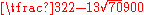
For the simplest integration problem stated above, i.e. with ,
,
the associated polynomials are Legendre polynomials, Pn(x), and the method is usually known as Gauss–Legendre quadrature. With the nth polynomial normalized to give Pn(1) = 1, the ith Gauss node, xi, is the ith root of Pn; its weight is given by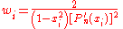
Some low-order rules for solving the integration problem are listed below.
After applying the Gaussian quadrature rule, the following approximation is:
ω into the integrand,
and allowing an interval other than [−1, 1].
That is, the problem is to calculate
for some choices of a, b, and ω.
For a = −1, b = 1, and ω(x) = 1,
the problem is the same as that considered above.
Other choices lead to other integration rules.
Some of these are tabulated below.
Equation numbers are given for Abramowitz and Stegun
(A & S).
 be a nontrivial polynomial of degree n such that

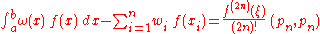
If we pick the n nodes xi to be the zeros of pn , then there exist n weights wi which make the Gauss-quadrature computed integral exact for all polynomials of degree 2n − 1 or less. Furthermore, all these nodes xi will lie in the open interval (a, b) .
The polynomial is said to be an orthogonal polynomial of degree n associated to the weight function
  . It is unique up to a constant normalization factor. The idea underlying the proof is that, because of its sufficiently low degree,
  can be divided by
  to produce a quotient
  of degree strictly lower than n, and a remainder
  of still lower degree, so that both will be orthogonal to
  , by the defining property of
  . Thus
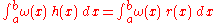 .
.
Because of the choice of nodes xi , the corresponding relation
holds also. The exactness of the computed integral for then follows from corresponding exactness for polynomials of degree only n or less (as is
  ). This (superficially less exacting) requirement can now be satisfied by choosing the weights wi equal to the integrals (using same weight function
  ) of the Lagrange basis polynomials
  of these particular n nodes xi.
 and weights
  of Gaussian quadrature rules, the fundamental tool is the three-term recurrence relation satisfied by the set of orthogonal polynomials associated to the corresponding weight function. For n points, these nodes and weights can be computed in O(n2) operations by the following algorithm.
If, for instance, is the monic orthogonal polynomial of degree n (the orthogonal polynomial of degree n with the highest degree coefficient equal to one), one can show that such orthogonal polynomials are related through the recurrence relation

From this, nodes and weights can be computed from the eigenvalues and eigenvectors of an associated linear algebra problem. This is usually named as the Golub–Welsch algorithm .
The starting idea comes from the observation that, if is a root of the orthogonal polynomial
  then, using the previous recurrence formula for
  and because
  , we have

where
and is the so-called Jacobi matrix:
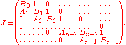
The nodes of gaussian quadrature can therefore be computed as the eigenvalues of a tridiagonal matrix.
For computing the weights and nodes, it is preferable to consider the symmetric tridiagonal matrix with elements
  and
and 
 and
and  are similar matrices and therefore have the same eigenvalues (the nodes). The weights can be computed from the corresponding eigenvectors: If
  is a normalized eigenvector (i.e., an eigenvector with euclidean norm equal to one) associated to the eigenvalue
  , the corresponding weight can be computed from
the first component of this eigenvector, namely:
where is the integral of the weight function
See, for instance, for further details.
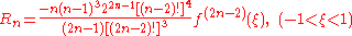
For an integrand which has 2n continuous derivatives,
for some ξ in (a, b), where pn is the orthogonal polynomial of degree n and where
In the important special case of ω(x) = 1, we have the error estimate
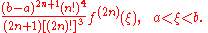
Stoer and Bulirsch remark that this error estimate is inconvenient in practice,
since it may be difficult to estimate the order 2n derivative,
and furthermore the actual error may be much less than a bound established by the derivative.
Another approach is to use two Gaussian quadrature rules of different orders,
and to estimate the error as the difference between the two results.
For this purpose, Gauss–Kronrod quadrature rules can be useful.
Important consequence of the above equation is that Gaussian quadrature of order n is accurate for all polynomials up to degree 2n–1.
the Gauss evaluation points of the new subintervals never coincide with the previous evaluation points (except at zero for odd numbers),
and thus the integrand must be evaluated at every point.
Gauss–Kronrod rules are extensions of Gauss quadrature rules generated by adding points to an
  -point rule in such a way that the resulting rule is of order
  .
.
This allows for computing higher-order estimates while re-using the function values of a lower-order estimate.
The difference between a Gauss quadrature rule and its Kronrod extension are often used as an estimate of the approximation error.
.
It is similar to Gaussian quadrature with the following differences:
Lobatto quadrature of function f(x) on interval [–1, +1]:
Abscissas: is the
  st zero of
  .
.
Weights: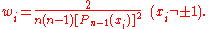
Remainder:
Numerical analysis
Numerical analysis is the study of algorithms that use numerical approximation for the problems of mathematical analysis ....
, a quadrature rule is an approximation of the definite integral
Integral
Integration is an important concept in mathematics and, together with its inverse, differentiation, is one of the two main operations in calculus...
of a function
Function (mathematics)
In mathematics, a function associates one quantity, the argument of the function, also known as the input, with another quantity, the value of the function, also known as the output. A function assigns exactly one output to each input. The argument and the value may be real numbers, but they can...
, usually stated as a weighted sum of function values at specified points within the domain of integration.
(See numerical integration
Numerical integration
In numerical analysis, numerical integration constitutes a broad family of algorithms for calculating the numerical value of a definite integral, and by extension, the term is also sometimes used to describe the numerical solution of differential equations. This article focuses on calculation of...
for more on quadrature
Quadrature (mathematics)
Quadrature — historical mathematical term which means calculating of the area. Quadrature problems have served as one of the main sources of mathematical analysis.- History :...
rules.)
An n-point Gaussian quadrature rule, named after Carl Friedrich Gauss
Carl Friedrich Gauss
Johann Carl Friedrich Gauss was a German mathematician and scientist who contributed significantly to many fields, including number theory, statistics, analysis, differential geometry, geodesy, geophysics, electrostatics, astronomy and optics.Sometimes referred to as the Princeps mathematicorum...
, is a quadrature rule constructed to yield an exact result for polynomial
Polynomial
In mathematics, a polynomial is an expression of finite length constructed from variables and constants, using only the operations of addition, subtraction, multiplication, and non-negative integer exponents...
s of degree 2n − 1 or less by a suitable choice of the points xi and weights wi for i = 1,...,n.
The domain of integration for such a rule is conventionally taken as [−1, 1],
so the rule is stated as
Gaussian quadrature as above will only produce accurate results if the function f(x) is well approximated by a polynomial function within the range [-1,1]. The method is not, for example, suitable for functions with singularities. However, if the integrated function can be written as
, where g(x) is approximately polynomial, and W(x) is known, then there are alternative weights
such thatCommon weighting functions include
(Gauss-Chebyshev) and
(Gauss-Hermite).It can be shown (see Press, et al., or Stoer and Bulirsch) that the evaluation points are just the roots of a polynomial
Polynomial
In mathematics, a polynomial is an expression of finite length constructed from variables and constants, using only the operations of addition, subtraction, multiplication, and non-negative integer exponents...
belonging to a class of orthogonal polynomials
Orthogonal polynomials
In mathematics, the classical orthogonal polynomials are the most widely used orthogonal polynomials, and consist of the Hermite polynomials, the Laguerre polynomials, the Jacobi polynomials together with their special cases the ultraspherical polynomials, the Chebyshev polynomials, and the...
.
Gauss–Legendre quadrature
For the simplest integration problem stated above, i.e. with
,the associated polynomials are Legendre polynomials, Pn(x), and the method is usually known as Gauss–Legendre quadrature. With the nth polynomial normalized to give Pn(1) = 1, the ith Gauss node, xi, is the ith root of Pn; its weight is given by
Some low-order rules for solving the integration problem are listed below.
| Number of points, n | Points, xi | Weights, wi |
|---|---|---|
| 1 | 0 | 2 |
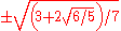
| 2 |  |
1 |
| 3 | 0 | 8⁄9 |
 |
5⁄9 | |
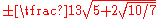
| 4 | 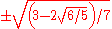 |
 |
 |
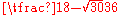 |
|
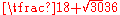
| 5 | 0 | 128⁄225 |
 |
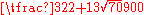 |
|
 |
 |
Change of interval
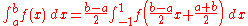
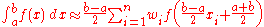
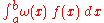
An integral over [a, b] must be changed into an integral over [−1, 1] before applying the Gaussian quadrature rule. This change of interval can be done in the following way:After applying the Gaussian quadrature rule, the following approximation is:
Other forms
The integration problem can be expressed in a slightly more general way by introducing a positive weight functionWeight function
A weight function is a mathematical device used when performing a sum, integral, or average in order to give some elements more "weight" or influence on the result than other elements in the same set. They occur frequently in statistics and analysis, and are closely related to the concept of a...
ω into the integrand,
and allowing an interval other than [−1, 1].
That is, the problem is to calculate
for some choices of a, b, and ω.
For a = −1, b = 1, and ω(x) = 1,
the problem is the same as that considered above.
Other choices lead to other integration rules.
Some of these are tabulated below.
Equation numbers are given for Abramowitz and Stegun
Abramowitz and Stegun
Abramowitz and Stegun is the informal name of a mathematical reference work edited by Milton Abramowitz and Irene Stegun of the U.S. National Bureau of Standards...
(A & S).
| Interval | ω(x) | Orthogonal polynomials | A & S | For more information, see ... |
|---|---|---|---|---|
| [−1, 1] |  |
Legendre polynomials | 25.4.29 | Section Gauss–Legendre quadrature, above |
| (−1, 1) | 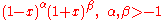 |
Jacobi polynomials Jacobi polynomials In mathematics, Jacobi polynomials are a class of classical orthogonal polynomials. They are orthogonal with respect to the weight ^\alpha ^\beta on the interval [-1, 1]... |
25.4.33 ( ) ) |
Gauss–Jacobi quadrature |
| (−1, 1) |  |
Chebyshev polynomials Chebyshev polynomials In mathematics the Chebyshev polynomials, named after Pafnuty Chebyshev, are a sequence of orthogonal polynomials which are related to de Moivre's formula and which can be defined recursively. One usually distinguishes between Chebyshev polynomials of the first kind which are denoted Tn and... (first kind) |
25.4.38 | Chebyshev–Gauss quadrature |
| [−1, 1] |  |
Chebyshev polynomials (second kind) | 25.4.40 | Chebyshev–Gauss quadrature |
| [0, ∞) |  |
Laguerre polynomials Laguerre polynomials In mathematics, the Laguerre polynomials, named after Edmond Laguerre ,are the canonical solutions of Laguerre's equation:x\,y + \,y' + n\,y = 0\,which is a second-order linear differential equation.... |
25.4.45 | Gauss–Laguerre quadrature |
| (−∞, ∞) |  |
Hermite polynomials Hermite polynomials In mathematics, the Hermite polynomials are a classical orthogonal polynomial sequence that arise in probability, such as the Edgeworth series; in combinatorics, as an example of an Appell sequence, obeying the umbral calculus; in numerical analysis as Gaussian quadrature; and in physics, where... |
25.4.46 | Gauss–Hermite quadrature |
Fundamental theorem
Let be a nontrivial polynomial of degree n such thatIf we pick the n nodes xi to be the zeros of pn , then there exist n weights wi which make the Gauss-quadrature computed integral exact for all polynomials
of degree 2n − 1 or less. Furthermore, all these nodes xi will lie in the open interval (a, b) .The polynomial
is said to be an orthogonal polynomial of degree n associated to the weight function . It is unique up to a constant normalization factor. The idea underlying the proof is that, because of its sufficiently low degree, can be divided by to produce a quotient of degree strictly lower than n, and a remainder of still lower degree, so that both will be orthogonal to , by the defining property of . Thus.Because of the choice of nodes xi , the corresponding relation
holds also. The exactness of the computed integral for
then follows from corresponding exactness for polynomials of degree only n or less (as is ). This (superficially less exacting) requirement can now be satisfied by choosing the weights wi equal to the integrals (using same weight function ) of the Lagrange basis polynomials of these particular n nodes xi.Computation of Gaussian quadrature rules
For computing the nodes and weights of Gaussian quadrature rules, the fundamental tool is the three-term recurrence relation satisfied by the set of orthogonal polynomials associated to the corresponding weight function. For n points, these nodes and weights can be computed in O(n2) operations by the following algorithm.If, for instance,
is the monic orthogonal polynomial of degree n (the orthogonal polynomial of degree n with the highest degree coefficient equal to one), one can show that such orthogonal polynomials are related through the recurrence relationRecurrence relation
In mathematics, a recurrence relation is an equation that recursively defines a sequence, once one or more initial terms are given: each further term of the sequence is defined as a function of the preceding terms....
From this, nodes and weights can be computed from the eigenvalues and eigenvectors of an associated linear algebra problem. This is usually named as the Golub–Welsch algorithm .
The starting idea comes from the observation that, if
is a root of the orthogonal polynomial then, using the previous recurrence formula for and because , we havewhere
and
is the so-called Jacobi matrix:The nodes of gaussian quadrature can therefore be computed as the eigenvalues of a tridiagonal matrix.
For computing the weights and nodes, it is preferable to consider the symmetric tridiagonal matrix
with elements and and are similar matrices and therefore have the same eigenvalues (the nodes). The weights can be computed from the corresponding eigenvectors: If is a normalized eigenvector (i.e., an eigenvector with euclidean norm equal to one) associated to the eigenvalue , the corresponding weight can be computed fromthe first component of this eigenvector, namely:
where
is the integral of the weight functionSee, for instance, for further details.
Error estimates
The error of a Gaussian quadrature rule can be stated as follows .For an integrand which has 2n continuous derivatives,
for some ξ in (a, b), where pn is the orthogonal polynomial of degree n and where
In the important special case of ω(x) = 1, we have the error estimate
Stoer and Bulirsch remark that this error estimate is inconvenient in practice,
since it may be difficult to estimate the order 2n derivative,
and furthermore the actual error may be much less than a bound established by the derivative.
Another approach is to use two Gaussian quadrature rules of different orders,
and to estimate the error as the difference between the two results.
For this purpose, Gauss–Kronrod quadrature rules can be useful.
Important consequence of the above equation is that Gaussian quadrature of order n is accurate for all polynomials up to degree 2n–1.
Gauss–Kronrod rules
If the interval [a, b] is subdivided,the Gauss evaluation points of the new subintervals never coincide with the previous evaluation points (except at zero for odd numbers),
and thus the integrand must be evaluated at every point.
Gauss–Kronrod rules are extensions of Gauss quadrature rules generated by adding
points to an -point rule in such a way that the resulting rule is of order .This allows for computing higher-order estimates while re-using the function values of a lower-order estimate.
The difference between a Gauss quadrature rule and its Kronrod extension are often used as an estimate of the approximation error.
Gauss–Lobatto rules
Also known as Lobatto quadrature , named after Dutch mathematician Rehuel LobattoRehuel Lobatto
Rehuel Lobatto was a Dutch mathematician. Lobatto was born in Amsterdam to a Portuguese Marrano family. As a schoolboy Lobatto already displayed remarkable talent for mathematics...
.
It is similar to Gaussian quadrature with the following differences:
- The integration points include the end points of the integration interval.
- It is accurate for polynomials up to degree 2n–3, where n is the number of integration points.
Lobatto quadrature of function f(x) on interval [–1, +1]:
Abscissas:
is the st zero of .Weights:
Remainder:
External links
- ALGLIB contains a collection of algorithms for numerical integration (in C# / C++ / Delphi / Visual Basic / etc.)
- GNU Scientific Library - includes CC (programming language)C is a general-purpose computer programming language developed between 1969 and 1973 by Dennis Ritchie at the Bell Telephone Laboratories for use with the Unix operating system....
version of QUADPACKQUADPACKQUADPACK is a FORTRAN 77 library for numerical integration of one-dimensional functions. It was included in the SLATEC Common Mathematical Library and is therefore in the public domain. The individual subprograms are also available on netlib....
algorithms (see also GNU Scientific LibraryGNU Scientific LibraryIn computing, the GNU Scientific Library is a software library written in the C programming language for numerical calculations in applied mathematics and science...
) - From Lobatto Quadrature to the Euler constant e
- Gaussian Quadrature Rule of Integration - Notes, PPT, Matlab, Mathematica, Maple, Mathcad at Holistic Numerical Methods Institute
- Legendre-Gauss Quadrature at MathWorld
- Gaussian Quadrature by Chris Maes and Anton Antonov, Wolfram Demonstrations ProjectWolfram Demonstrations ProjectThe Wolfram Demonstrations Project is hosted by Wolfram Research, whose stated goal is to bring computational exploration to the widest possible audience. It consists of an organized, open-source collection of small interactive programs called Demonstrations, which are meant to visually and...
. - Tabulated weights and abscissae with Mathematica source code, high precision (16 and 256 decimal places) Legendre-Gaussian quadrature weights and abscissas, for n=2 through n=64, with Mathematica source code.
- High-precision abscissas and weights for Gaussian Quadrature n = 2, ..., 20, 32, 64, 100, 128, 256, 512, 1024 with open source libraries for C/C++ and Matlab.