
Fourier optics
Encyclopedia
Fourier optics is the study of classical optics
using Fourier transform
s and can be seen as the dual of the Huygens-Fresnel principle
. In the latter case, the wave is regarded as a superposition of expanding spherical waves which radiate outward from actual (physically identifiable) current sources via a Green's function
relationship (see Double-slit experiment
). In Fourier optics, by contrast, the wave is regarded as a superposition of plane waves which are not related to any identifiable sources; instead they are the natural modes of the propagation medium itself. A curved phasefront may be synthesized from an infinite number of these "natural modes" i.e., from plane wave phasefronts oriented in different directions in space. Far from its sources, an expanding spherical wave is locally tangent to a planar phase front (a single plane wave out of the infinite spectrum), which is transverse to the radial direction of propagation. In this case, a Fraunhofer diffraction
pattern is created, which emanates from a single spherical wave phase center. In the near field, no single well-defined spherical wave phase center exists, so the wavefront isn't locally tangent to a spherical ball. In this case, a Fresnel diffraction
pattern would be created, which emanates from an extended source, consisting of a distribution of (physically identifiable) spherical wave sources in space. In the near field, a full spectrum of plane waves is necessary to represent the Fresnel near-field wave, even locally. A "wide" wave
moving forward (like an expanding ocean wave coming toward the shore) can be regarded as an infinite number of "plane wave modes", all of which could (when they collide with something in the way) scatter independently of one other. These mathematical simplifications and calculations are the realm of Fourier analysis and synthesis – together, they can describe what happens when light passes through various slits, lenses or mirrors curved one way or the other, or is fully or partially reflected. Fourier optics forms much of the theory behind image processing techniques
, as well as finding applications where information needs to be extracted from optical sources such as in quantum optics
. To put it in a slightly more complex way, similar to the concept of frequency
and time
used in traditional Fourier transform theory
, Fourier optics makes use of the spatial frequency
domain (kx, ky) as the conjugate of the spatial (x,y) domain. Terms and concepts such as transform theory, spectrum, bandwidth, window functions and sampling from one dimensional signal processing
are commonly used.

where

represents position in three dimensional space, and t represents time.
(valid in source-free regions):

where u(r,t) is a real valued
Cartesian component of an electromagnetic wave propagating through free space.
/wavelength
/color
(as from a laser) is assumed, then the time-harmonic
(frequency-domain) form of the optical field is given as:

where is in general a complex quantity, with separate amplitude and phase.
The time-domain field is related to the frequency domain field via the equation,
 .
.
Substituting this expression into the wave equation yields the time-independent form of the wave equation, also known as the Helmholtz equation
:

where
is the wave number, j is the imaginary unit
, and ψ(r) is the time-independent, complex-valued
component of the propagating wave. Note that the propagation constant, k, and the frequency, , are linearly related to one another, a typical characteristic of transverse electromagnetic (TEM) waves in homogeneous media.

where

is the wave vector
, and

is the wave number. Next, using the paraxial approximation
, it is assumed that

or equivalently,

where θ is the angle between the wave vector k and the z-axis.
As a result,
and

where
is the transverse Laplacian operator, shown here in Cartesian coordinates.
In this section, we won't go all the way back to Maxwell's equations, but will start instead with the homogeneous Helmholtz equation (valid in source-free media), which is one level of refinement up from Maxwell's equations (Scott [1998]). From this equation, we'll show how infinite uniform plane waves comprise one field solution (out of many possible) in free space. These uniform plane waves form the basis for understanding Fourier optics.
The plane wave
spectrum concept is the basic foundation of Fourier Optics. The plane wave spectrum is a continuous spectrum of uniform plane waves, and there is one plane wave component in the spectrum for every tangent point on the far-field phase front. The amplitude of that plane wave component would be the amplitude of the optical field at that tangent point. Again, this is true only in the far field, defined as: Range = 2 D2 / λ where D is the maximum linear extent of the optical sources and λ is the wavelength (Scott [1998]). The plane wave spectrum is often regarded as being discrete for certain types of periodic gratings, though in reality, the spectra from gratings are continuous as well, since no physical device can have the infinite extent required to produce a true line spectrum.
As in the case of electrical signals, bandwidth is a measure of how finely detailed an image is; the finer the detail, the greater the bandwidth required to represent it. A DC electrical signal is constant and has no oscillations; a plane wave propagating parallel to the optic axis has constant value in any x-y plane, and therefore is analogous to the (constant) DC component of an electrical signal. Bandwidth in electrical signals relates to the difference between the highest and lowest frequencies present in the spectrum of the signal. For optical systems, bandwidth also relates to spatial frequency content (spatial bandwidth), but it also has a secondary meaning. It also measures how far from the optic axis the corresponding plane waves are tilted, and so this type of bandwidth is often referred to also as angular bandwidth. It takes more frequency bandwidth to produce a short pulse in an electrical circuit, and more angular (or, spatial frequency) bandwidth to produce a sharp spot in an optical system (see discussion related to Point spread function
).
The plane wave spectrum arises naturally as the eigenfunction
or "natural mode" solution to the homogeneous electromagnetic wave equation
in rectangular coordinates (see also Electromagnetic radiation
, which derives the wave equation from Maxwell's equations in source-free media, or Scott [1998]). In the frequency domain
, with an assumed (engineering) time convention of ,
,
the homogeneous electromagnetic wave equation is known as the Helmholtz equation
and takes the form:
where u = x, y, z and k = 2π/λ is the wavenumber
of the medium.
solution, in physics as a "natural mode" solution and in electrical circuit theory as the "zero-input response." This is a concept that spans a wide range of physical disciplines. Common physical examples of resonant natural modes would include the resonant vibrational modes of stringed instruments (1D), percussion instruments (2D) or the former Tacoma Narrows bridge
(3D). Examples of propagating natural modes would include waveguide
modes, optical fiber
modes, solitons
and Bloch wave
s. Infinite homogeneous media admit the rectangular, circular and spherical harmonic solutions to the Helmholtz equation, depending on the coordinate system under consideration. The propagating plane waves we'll study in this article are perhaps the simplest type of propagating waves found in any type of media.
There is a striking similarity between the Helmholtz equation (2.0) above, which may be written
and the usual equation for the eigenvalues/eigenvectors
of a square matrix, A,
particularly since both the scalar Laplacian, and the matrix, A are linear operators on their respective function/vector spaces (the minus sign in the second equation is, for all intents and purposes, immaterial; the plus sign in the first equation however is significant). It is perhaps worthwhile to note that both the eigenfunction and eigenvector solutions to these two equations respectively, often yield an orthogonal set of functions/vectors which span (i.e., form a basis set for) the function/vector spaces under consideration. The interested reader may investigate other functional linear operators which give rise to different kinds of orthogonal eigenfunctions such as Legendre polynomials, Chebyshev polynomials
and Hermite polynomials
.
In the matrix case, eigenvalues may be found by setting the determinant of the matrix equal to zero, i.e. finding where the matrix has no inverse. Finite matrices have only a finite number of eigenvalues/eigenvectors, whereas linear operators can have a countably infinite number of eigenvalues/eigenfunctions (in confined regions) or uncountably infinite (continuous) spectra of solutions, as in unbounded regions.
In certain physics applications, it is often the case that the elements of a matrix will be functions of frequency and wavenumber, and the matrix will be non-singular for most combinations of frequency and wavenumber, but will also be singular for certain other combinations. By finding which combinations of frequency and wavenumber drive the determinant of the matrix to zero, the propagation characteristics of the medium may be determined. Relations of this type, between frequency and wavenumber, are known as dispersion relations and some physical systems may admit many different kinds of dispersion relations. An example from electromagnetics is the ordinary waveguide, which may admit numerous dispersion relations, each associated with a unique mode of the waveguide. Each propagation mode of the waveguide is known as an eigenfunction
solution (or eigenmode solution) to Maxwell's equations in the waveguide. Free space also admits eigenmode (natural mode) solutions (known more commonly as plane waves), but with the distinction that for any given frequency, free space admits a continuous modal spectrum, whereas waveguides have a discrete mode spectrum. In this case the dispersion relation is linear, as in section 1.2.
for partial differential equations. This principle says that in separable orthogonal coordinates
, an elementary product solution to this wave equation may be constructed of the following form:
i.e., as the product of a function of x, times a function of y, times a function of z. If this elementary product solution is substituted into the wave equation (2.0), using the scalar Laplacian
in rectangular coordinates:
then the following equation for the 3 individual functions is obtained
which is readliy rearranged into the form:
It may now be argued that each of the quotients in the equation above must, of necessity, be constant. For, say the first quotient is not constant, and is a function of x. None of the other terms in the equation has any dependence on the variable x. Therefore, the first term may not have any x-dependence either; it must be constant. The constant is denoted as -kx². Reasoning in a similar way for the y and z quotients, three ordinary differential equations are obtained for the fx, fy and fz, along with one separation condition:
Each of these 3 differential equations has the same solution: sines, cosines or complex exponentials. We'll go with the complex exponential for notational simplicity, compatibility with usual FT notation, and the fact that a two-sided integral of complex exponentials picks up both the sine and cosine contributions. As a result, the elementary product solution for Eu is:
which represents a propagating or exponentially decaying uniform plane wave solution to the homogeneous wave equation. The - sign is used for a wave propagating/decaying in the +z direction and the + sign is used for a wave propagating/decaying in the -z direction (this follows the engineering time convention, which assumes an ejωt time dependence). This field represents a propagating plane wave when the quantity under the radical is positive, and an exponentially decaying wave when it is negative (in passive media, the root with a non-positive imaginary part must always be chosen, to represent uniform propagation or decay, but not amplification).
Product solutions to the Helmholtz equation are also readily obtained in cylindrical
and spherical coordinates
, yielding cylindrical and spherical harmonics (with the remaining separable coordinate systems being used much less frequently).
where the integrals extend from minus infinity to infinity.
This plane wave spectrum representation of the electromagnetic field is the basic foundation of Fourier Optics (this point cannot be emphasized strongly enough), because when z=0, the equation above simply becomes a Fourier transform (FT) relationship between the field and its plane wave content (hence the name, "Fourier optics").
All spatial dependence of the individual plane wave components is described explicitly via the exponential functions. The coefficients of the exponentials are only functions of spatial wavenumber kx, ky, just as in ordinary Fourier analysis and Fourier transform
s.
the plane waves are evanescent (decaying), so that any spatial frequency content in an object plane transparency which is finer than one wavelength will not be transferred over to the image plane, simply because the plane waves corresponding to that content cannot propagate. In connection with lithography of electronic components, this phenomenon is known as the diffraction limit and is the reason why light of progressively higher frequency (smaller wavelength) is required for etching progressively finer features in integrated circuits.
which clearly indicates that the field at (x,y,z) is directly proportional to the spectral component in the direction of (x,y,z), where,
and
Stated another way, the radiation pattern of any planar field distribution is the FT of that source distribution (see Huygens-Fresnel principle
, wherein the same equation is developed using a Green's function
approach). Note that this is NOT a plane wave, as many might think. The radial dependence is a spherical wave - both in magnitude and phase - whose local amplitude is the FT of the source plane distribution at that far field angle. The plane wave spectrum has nothing to do with saying that the field behaves something like a plane wave for far distances.
Equation (2.2) above is critical to making the connection between spatial bandwidth (on the one hand) and angular bandwidth (on the other), in the far field. Note that the term "far field" usually means we're talking about a converging or diverging spherical wave with a pretty well defined phase center. The connection between spatial and angular bandwidth in the far field is essential in understanding the low pass filtering property of thin lenses. See section 5.1.3 for the condition defining the far field region.
Once the concept of angular bandwidth is understood, the optical scientist can "jump back and forth" between the spatial and spectral domains to quickly gain insights which would ordinarily not be so readily available just through spatial domain or ray optics considerations alone. For example, any source bandwidth which lies past the edge angle to the first lens (this edge angle sets the bandwidth of the optical system) will not be captured by the system to be processed.
As a side note, electromagnetics scientists have devised an alternative means for calculating the far zone electric field which does not involve stationary phase integration. They have devised a concept known as "fictitious magnetic currents" usually denoted by M, and defined as
In this equation, it is assumed that the unit vector in the z-direction points into the half-space where the far field calculations will be made. These equivalent magnetic currents are obtained using equivalence principles which, in the case of an infinite planar interface, allow any electric currents, J to be "imaged away" while the fictitious magnetic currents are obtained from twice the aperture electric field (see Scott [1998]). Then the radiated electric field is calculated from the magnetic currents using an equation similar to the equation for the magnetic field radiated by an electric current. In this way, a vector equation is obtained for the radiated electric field in terms of the aperture electric field and the derivation requires no use of stationary phase ideas.
which is identical to the equation for the Euclidean metric in three-dimensional configuration space, suggests the notion of a k-vector
in three-dimensional "k-space", defined (for propagating plane waves) in rectangular coordinates as:
and in the spherical coordinate system
as
Use will be made of these spherical coordinate system relations in the next section.
The notion of k-space is central to many disciplines in engineering and physics, especially in the study of periodic volumes, such as in crystallography and the band theory of semiconductor materials.

Synthesis Equation (reconstructing the function from its spectrum):
Note: the normalizing factor of: is present whenever angular frequency (radians) is used, but not when ordinary frequency (cycles) is used.
The impulse response of an optical imaging system is the output plane field which is produced when an ideal mathematical point source of light is placed in the input plane (usually on-axis). In practice, it is not necessary to have an ideal point source in order to determine an exact impulse response. This is because any source bandwidth which lies outside the bandwidth of the system won't matter anyway (since it cannot even be captured by the optical system), so therefore it's not necessary in determining the impulse response. The source only needs to have at least as much (angular) bandwidth as the optical system.
Optical systems typically fall into one of two different categories. The first is the ordinary focused optical imaging system, wherein the input plane is called the object plane and the output plane is called the image plane. The field in the image plane is desired to be a high-quality reproduction of the field in the object plane. In this case, the impulse response of the optical system is desired to approximate a 2D delta function, at the same location (or a linearly scaled location) in the output plane corresponding to the location of the impulse in the input plane. The actual impulse response typically resembles an Airy function, whose radius is on the order of the wavelength of the light used. In this case, the impulse response is typically referred to as a point spread function
, since the mathematical point of light in the object plane has been spread out into an Airy function in the image plane.
The second type is the optical image processing system, in which a significant feature in the input plane field is to be located and isolated. In this case, the impulse response of the system is desired to be a close replica (picture) of that feature which is being searched for in the input plane field, so that a convolution of the impulse response (an image of the desired feature) against the input plane field will produce a bright spot at the feature location in the output plane. It is this latter type of optical image processing system that is the subject of this section. Section 5.2 presents one hardware implementation of the optical image processing operations described in this section.


i.e.,

The alert reader will note that the integral above tacitly assumes that the impulse response is NOT a function of the position (x',y') of the impulse of light in the input plane (if this were not the case, this type of convolution would not be possible). This property is known as shift invariance (Scott [1998]). No optical system is perfectly shift invariant: as the ideal, mathematical point of light is scanned away from the optic axis, aberrations will eventually degrade the impulse response (known as a coma
in focused imaging systems). However, high quality optical systems are often "shift invariant enough" over certain regions of the input plane that we may regard the impulse response as being a function of only the difference between input and output plane coordinates, and thereby use the equation above with impunity.
Also, this equation assumes unit magnification. If magnification is present, then eqn. (4.1) becomes

which basically translates the impulse response function, hM, from x' to x=Mx'. In (4.2), hM will be a magnified version of the impulse response function h of a similar, unmagnified system, so that hM(x,y) =h(x/M,y/M).
exists in the time domain, but not in the spatial domain. Causality means that the impulse response h(t - t') of an electrical system, due to an impulse applied at time t', must of necessity be zero for all times t such that t - t' < 0.
Obtaining the convolution representation of the system response requires representing the input signal as a weighted superposition over a train of impulse functions by using the sifting property of Dirac delta function
s.

It is then presumed that the system under consideration is linear, that is to say that the output of the system due to two different inputs (possibly at two different times) is the sum of the individual outputs of the system to the two inputs, when introduced individually. Thus the optical system may contain no nonlinear materials nor active devices (except possibly, extremely linear active devices). The output of the system, for a single delta function input is defined as the impulse response of the system, h(t - t'). And, by our linearity assumption (i.e., that the output of system to a pulse train input is the sum of the outputs due to each individual pulse), we can now say that the general input function f(t) produces the output:

where h(t - t') is the (impulse) response of the linear system to the delta function input δ(t - t'), applied at time t'. This is where the convolution equation above comes from. The convolution equation is useful because it is often much easier to find the response of a system to a delta function input - and then perform the convolution above to find the response to an arbitrary input - than it is to try to find the response to the arbitrary input directly. Also, the impulse response (in either time or frequency domains) usually yields insight to relevant figures of merit of the system. In the case of most lenses, the point spread function (PSF) is a pretty common figure of merit for evaluation purposes.
The same logic is used in connection with the Huygens-Fresnel principle
, or Stratton-Chu formulation, wherein the "impulse response" is referred to as the Green's function
of the system. So the spatial domain operation of a linear optical system is analogous in this way to the Huygens-Fresnel principle.

where
 is the spectrum of the output signal
 is the system transfer function
 is the spectrum of the input signal
In like fashion, (4.1) may be Fourier transformed to yield:

Once again it may be noted from the discussion on the Abbe sine condition
, that this equation assumes unit magnification.
This equation takes on its real meaning when the Fourier transform, is associated with the coefficient of the plane wave whose transverse wavenumbers are
  . Thus, the input-plane plane wave spectrum is transformed into the output-plane plane wave spectrum through the multiplicative action of the system transfer function. It is at this stage of understanding that the previous background on the plane wave spectrum becomes invaluable to the conceptualization of Fourier optical systems.
The Fourier transform
properties of a lens
provide numerous applications in optical signal processing such as spatial filtering, optical correlation and computer generated holograms.
Fourier optical theory is used in interferometry
, optical tweezers
, atom traps
, and quantum computing. Concepts of Fourier optics are used to reconstruct the phase
of light intensity in the spatial frequency plane (see adaptive-additive algorithm
).
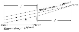
, then its Fourier transform
will be formed one focal length behind the lens. Consider the figure to the right (click to enlarge)
 In this figure, a plane wave incident from the left is assumed. The transmittance function in the front focal plane (i.e., Plane 1) spatially modulates the incident plane wave in magnitude and phase, like on the left-hand side of eqn. (2.1) (specified to z=0), and in so doing, produces a spectrum of plane waves corresponding to the FT of the transmittance function, like on the right-hand side of eqn. (2.1) (for z>0). The various plane wave components propagate at different tilt angles with respect to the optic axis of the lens (i.e., the horizontal axis). The finer the features in the transparency, the broader the angular bandwidth of the plane wave spectrum. We'll consider one such plane wave component, propagating at angle θ with respect to the optic axis. It is assumed that θ is small (paraxial approximation
), so that
and
and
In the figure, the plane wave phase, moving horizontally from the front focal plane to the lens plane, is
and the spherical wave phase from the lens to the spot in the back focal plane is:
and the sum of the two path lengths is f (1 + θ2/2 + 1 - θ2/2) = 2f i.e., it is a constant value, independent of tilt angle, θ, for paraxial plane waves. Each paraxial plane wave component of the field in the front focal plane appears as a Point spread function
spot in the back focal plane, with an intensity and phase equal to the intensity and phase of the original plane wave component in the front focal plane. In other words, the field in the back focal plane is the Fourier transform
of the field in the front focal plane.
All FT components are computed simultaneously - in parallel - at the speed of light. As an example, light travels at a speed of roughly 1 ft (0.3048 m). / ns, so if a lens has a 1 ft (0.3048 m). focal length, an entire 2D FT can be computed in about 2 ns (2 x 10⁻⁹ seconds). If the focal length is 1 in., then the time is under 200 ps. No electronic computer can compete with these kinds of numbers or perhaps ever hope to, although new supercomputers such as the petaflop IBM Roadrunner may actually prove faster than optics, as improbable as that may seem. However, their speed is obtained by combining numerous computers which, individually, are still slower than optics. The disadvantage of the optical FT is that, as the derivation shows, the FT relationship only holds for paraxial plane waves, so this FT "computer" is inherently bandlimited. On the other hand, since the wavelength of visible light is so minute in relation to even the smallest visible feature dimensions in the image i.e.,
(for all kx, ky within the spatial bandwidth of the image, so that kz is nearly equal to k), the paraxial approximation is not terribly limiting in practice. And, of course, this is an analog - not a digital - computer, so precision is limited. Also, phase can be challenging to extract; often it is inferred interferometrically.
Optical processing is especially useful in real time applications where rapid processing of massive amounts of 2D data is required, particularly in relation to pattern recognition.
Whenever a function is discontinuously truncated in one FT domain, broadening and rippling are introduced in the other FT domain. A perfect example from optics is in connection with the Point spread function
, which for on-axis plane wave illumination of a quadratic lens (with circular aperture), is an Airy function, J1(x)/x. Literally, the point source has been "spread out" (with ripples added), to form the Airy point spread function (as the result of truncation of the plane wave spectrum by the finite aperture of the lens). This source of error is known as Gibbs phenomenon
and it may be mitigated by simply ensuring that all significant content lies near the center of the transparency, or through the use of window function
s which smoothly taper the field to zero at the frame boundaries. By the convolution theorem, the FT of an arbitrary transparency function - multiplied (or truncated) by an aperture function - is equal to the FT of the non-truncated transparency function convolved against the FT of the aperture function, which in this case becomes a type of "Greens function" or "impulse response function" in the spectral domain. Therefore, the image of a circular lens is equal to the object plane function convolved against the Airy function (the FT of a circular aperture function is J1(x)/x and the FT of a rectangular aperture function is a product of sinc functions, sin x/x).
This issue brings up perhaps the predominant difficulty with Fourier analysis, namely that the input-plane function, defined over a finite support (i.e., over its own finite aperture), is being approximated with other functions (sinusiods) which have infinite support (i.e., they are defined over the entire infinite x-y plane). This is unbelievably inefficient computationally, and is the principal reason why wavelet
s were conceived, that is to represent a function (defiined on a finite interval or area) in terms of oscillatory functions which are also defined over finite intervals or areas. Thus, instead of getting the frequency content of the entire image all at once (along with the frequency content of the entire rest of the x-y plane, over which the image has zero value), the result is instead the frequency content of different parts of the image, which is usually much simpler. Unfortunately, wavelets in the x-y plane don't correspond to any known type of propagating wave function, in the same way that Fourier's sinusoids (in the x-y plane) correspond to plane wave functions in three dimensions. However, the FTs of most wavelets are well known and could possibly be shown to be equivalent to some useful type of propagating field.
On the other hand, Sinc functions and Airy functions - which are not only the point spread functions of rectangular and circular apertures, respectively, but are also cardinal functions commonly used for functional decomposition in interpolation/sampling theory [Scott 1990] - do correspond to converging or diverging spherical waves, and therefore could potentially be implemented as a whole new functional decomposition of the object plane function, thereby leading to another point of view similar in nature to Fourier optics. This would basically be the same as conventional ray optics, but with diffraction effects included. In this case, each point spread function would be a type of "smooth pixel," in much the same way that a soliton on a fiber is a "smooth pulse."
Perhaps a lens figure-of-merit in this "point spread function" viewpoint would be to ask how well a lens transforms an Airy function in the object plane into an Airy function in the image plane, as a function of radial distance from the optic axis, or as a function of the size of the object plane Airy function. This is kind of like the Point spread function
, except now we're really looking at it as a kind of input-to-output plane transfer function (like MTF), and not so much in absolute terms, relative to a perfect point. Similarly, Gaussian wavelets, which would correspond to the waist of a propagating Gaussian beam, could also potentially be used in still another functional decomposition of the object plane field.
Since the lens is in the far field of any PSF spot, the field incident on the lens from the spot may be regarded as being a spherical wave, as in eqn. (2.2), not as a plane wave spectrum, as in eqn. (2.1). On the other hand, the lens is in the near field of the entire input plane transparency, therefore eqn. (2.1) - the full plane wave spectrum - accurately represents the field incident on the lens from that larger, extended source.
). Consider a "small" light source located on-axis in the object plane of the lens. It is assumed that the source is small enough that, by the far-field criterion, the lens is in the far field of the "small" source. Then, the field radiated by the small source is a spherical wave which is modulated by the FT of the source distribution, as in eqn. (2.2), Then, the lens passes - from the object plane over onto the image plane - only that portion of the radiated spherical wave which lies inside the edge angle of the lens. In this far-field case, truncation of the radiated spherical wave is equivalent to truncation of the plane wave spectrum of the small source. So, the plane wave components in this far-field spherical wave, which lie beyond the edge angle of the lens, are not captured by the lens and are not transferred over to the image plane. Note: this logic is valid only for small sources, such that the lens is in the far field region of the source, according to the 2 D2 / λ criterion mentioned previously. If an object plane transparency is imagined as a summation over small sources (as in the Whittaker-Shannon interpolation formula, Scott [1990]), each of which has its spectrum truncated in this fashion, then every point of the entire object plane transparency suffers the same effects of this low pass filtering.
Loss of the high (spatial) frequency content causes blurring and loss of sharpness (see discussion related to Point spread function
). Bandwidth truncation causes a (fictitious, mathematical, ideal) point source in the object plane to be blurred (or, spread out) in the image plane, giving rise to the term, "point spread function." Whenever bandwidth is expanded or contracted, image size is typically contracted or expanded accordingly, in such a way that the space-bandwidth product remains constant, by Heisenberg's principle (Scott [1998] and Abbe sine condition
).
and convolution
, this device - 4 focal lengths long - actually serves a wide variety of image processing operations that go well beyond what its name implies. A diagram of a typical 4F correlator is shown in the figure below (click to enlarge). This device may be readily understood by combining the plane wave spectrum representation of the electric field (section 2) with the Fourier transforming property of quadratic lenses (section 5.1) to yield the optical image processing operations described in section 4.
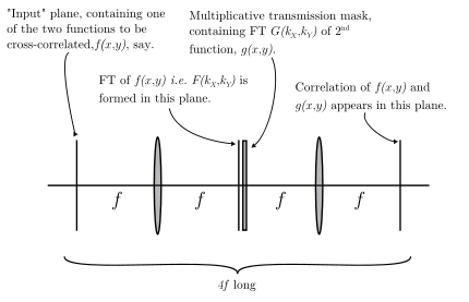 The 4F correlator is based on the convolution theorem
from Fourier transform
theory, which states that convolution
in the spatial (x,y) domain is equivalent to direct multiplication in the spatial frequency (kx, ky) domain (aka: spectral domain). Once again, a plane wave is assumed incident from the left and a transparency containing one 2D function, f(x,y), is placed in the input plane of the correlator, located one focal length in front of the first lens. The transparency spatially modulates the incident plane wave in magnitude and phase, like on the left-hand side of eqn. (2.1), and in so doing, produces a spectrum of plane waves corresponding to the FT of the transmittance function, like on the right-hand side of eqn. (2.1). That spectrum is then formed as an "image" one focal length behind the first lens, as shown. A transmission mask containing the FT of the second function, g(x,y), is placed in this same plane, one focal length behind the first lens, causing the transmission through the mask to be equal to the product, F(kx,ky) x G(kx,ky). This product now lies in the "input plane" of the second lens (one focal length in front), so that the FT of this product (i.e., the convolution
of f(x,y) and g(x,y)), is formed in the back focal plane of the second lens.
If an ideal, mathematical point source of light is placed on-axis in the input plane of the first lens, then there will be a uniform, collimated field produced in the output plane of the first lens. When this uniform, collimated field is multiplied by the FT plane mask, and then Fourier transformed by the second lens, the output plane field (which in this case is the impulse response of the correlator) is just our correlating function, g(x,y). In practical applications, g(x,y) will be some type of feature which must be identified and located within the input plane field (see Scott [1998]). In military applications, this feature may be a tank, ship or airplane which must be quickly identified within some more complex scene.
The 4F correlator is an excellent device for illustrating the "systems" aspects of optical instruments, alluded to in section 4 above. The FT plane mask function, G(kx,ky) is the system transfer function of the correlator, which we'd in general denote as H(kx,ky), and it is the FT of the impulse response function of the correlator, h(x,y) which is just our correlating function g(x,y). And, as mentioned above, the impulse response of the correlator is just a picture of the feature we're trying to find in the input image. In the 4F correlator, the system transfer function H(kx,ky) is directly multiplied against the spectrum F(kx,ky) of the input function, to produce the spectrum of the output function. This is how electrical signal processing systems operate on 1D temporal signals.
or Stratton-Chu viewpoints, the electric field is represented as a superposition of point sources, each one of which gives rise to a Green's function
field. The total field is then the weighted sum of all of the individual Greens function fields. That seems to be the most natural way of viewing the electric field for most people - no doubt because most of us have, at one time or another, drawn out the circles with protractor and paper, much the same way Thomas Young did in his classic paper on the Double-slit experiment
. However, it is by no means the only way to represent the electric field, which may also be represented as a spectrum of sinusoidally varying plane waves. In addition, Frits Zernike proposed still another functional decomposition
based on his Zernike polynomials
, defined on the unit disc. The third-order (and lower) Zernike polynomials correspond to the normal lens aberrations. And still another functional decomposition could be made in terms of Sinc functions and Airy functions, as in the Whittaker-Shannon interpolation formula and the Nyquist-Shannon sampling theorem. All of these functional decompositions have utility in different circumstances. The optical scientist having access to these various representational forms has available a richer insight to the nature of these marvelous fields and their properties. Embrace these different ways of looking at the field, rather than viewing them as being in any way conflicting or contradictory.
expansions and functional decomposition
, both briefly alluded to in this Wikipedia article, are not completely independent. The eigenfunction expansions to certain linear operators defined over a given domain, will often yield a countably infinite set of orthogonal functions
which will span that domain. Depending on the operator and the dimensionality (and shape, and boundary conditions) of its domain, many different types of functional decompositions are, in principle, possible.
-
Optics
Optics is the branch of physics which involves the behavior and properties of light, including its interactions with matter and the construction of instruments that use or detect it. Optics usually describes the behavior of visible, ultraviolet, and infrared light...
using Fourier transform
Fourier transform
In mathematics, Fourier analysis is a subject area which grew from the study of Fourier series. The subject began with the study of the way general functions may be represented by sums of simpler trigonometric functions...
s and can be seen as the dual of the Huygens-Fresnel principle
Huygens-Fresnel principle
The Huygens–Fresnel principle is a method of analysis applied to problems of wave propagation both in the far-field limit and in near-field diffraction.-History:...
. In the latter case, the wave is regarded as a superposition of expanding spherical waves which radiate outward from actual (physically identifiable) current sources via a Green's function
Green's function
In mathematics, a Green's function is a type of function used to solve inhomogeneous differential equations subject to specific initial conditions or boundary conditions...
relationship (see Double-slit experiment
Double-slit experiment
The double-slit experiment, sometimes called Young's experiment, is a demonstration that matter and energy can display characteristics of both waves and particles...
). In Fourier optics, by contrast, the wave is regarded as a superposition of plane waves which are not related to any identifiable sources; instead they are the natural modes of the propagation medium itself. A curved phasefront may be synthesized from an infinite number of these "natural modes" i.e., from plane wave phasefronts oriented in different directions in space. Far from its sources, an expanding spherical wave is locally tangent to a planar phase front (a single plane wave out of the infinite spectrum), which is transverse to the radial direction of propagation. In this case, a Fraunhofer diffraction
Fraunhofer diffraction
In optics, the Fraunhofer diffraction equation is used to model the diffraction of waves when the diffraction pattern is viewed at a long distance from the diffracting object, and also when it is viewed at the focal plane of an imaging lens....
pattern is created, which emanates from a single spherical wave phase center. In the near field, no single well-defined spherical wave phase center exists, so the wavefront isn't locally tangent to a spherical ball. In this case, a Fresnel diffraction
Fresnel diffraction
In optics, the Fresnel diffraction equation for near-field diffraction, is an approximation of Kirchhoff-Fresnel diffraction that can be applied to the propagation of waves in the near field....
pattern would be created, which emanates from an extended source, consisting of a distribution of (physically identifiable) spherical wave sources in space. In the near field, a full spectrum of plane waves is necessary to represent the Fresnel near-field wave, even locally. A "wide" wave
Wave
In physics, a wave is a disturbance that travels through space and time, accompanied by the transfer of energy.Waves travel and the wave motion transfers energy from one point to another, often with no permanent displacement of the particles of the medium—that is, with little or no associated mass...
moving forward (like an expanding ocean wave coming toward the shore) can be regarded as an infinite number of "plane wave modes", all of which could (when they collide with something in the way) scatter independently of one other. These mathematical simplifications and calculations are the realm of Fourier analysis and synthesis – together, they can describe what happens when light passes through various slits, lenses or mirrors curved one way or the other, or is fully or partially reflected. Fourier optics forms much of the theory behind image processing techniques
Image processing
In electrical engineering and computer science, image processing is any form of signal processing for which the input is an image, such as a photograph or video frame; the output of image processing may be either an image or, a set of characteristics or parameters related to the image...
, as well as finding applications where information needs to be extracted from optical sources such as in quantum optics
Quantum optics
Quantum optics is a field of research in physics, dealing with the application of quantum mechanics to phenomena involving light and its interactions with matter.- History of quantum optics :...
. To put it in a slightly more complex way, similar to the concept of frequency
Frequency
Frequency is the number of occurrences of a repeating event per unit time. It is also referred to as temporal frequency.The period is the duration of one cycle in a repeating event, so the period is the reciprocal of the frequency...
and time
Time in physics
Time in physics is defined by its measurement: time is what a clock reads. It is a scalar quantity and, like length, mass, and charge, is usually described as a fundamental quantity. Time can be combined mathematically with other physical quantities to derive other concepts such as motion, kinetic...
used in traditional Fourier transform theory
Fourier transform
In mathematics, Fourier analysis is a subject area which grew from the study of Fourier series. The subject began with the study of the way general functions may be represented by sums of simpler trigonometric functions...
, Fourier optics makes use of the spatial frequency
Spatial frequency
In mathematics, physics, and engineering, spatial frequency is a characteristic of any structure that is periodic across position in space. The spatial frequency is a measure of how often sinusoidal components of the structure repeat per unit of distance. The SI unit of spatial frequency is...
domain (kx, ky) as the conjugate of the spatial (x,y) domain. Terms and concepts such as transform theory, spectrum, bandwidth, window functions and sampling from one dimensional signal processing
Signal processing
Signal processing is an area of systems engineering, electrical engineering and applied mathematics that deals with operations on or analysis of signals, in either discrete or continuous time...
are commonly used.
Overview of light propagation in homogeneous, source-free media
Light can be described as a waveform propagating through free space (vacuum) or a material medium (such as air or glass). Mathematically, the (real valued) amplitude of one wave component is represented by a scalar wave function u that depends on both space and time:where
represents position in three dimensional space, and t represents time.
The Wave Equation in the Time Domain
Fourier optics begins with the homogeneous, scalar wave equationWave equation
The wave equation is an important second-order linear partial differential equation for the description of waves – as they occur in physics – such as sound waves, light waves and water waves. It arises in fields like acoustics, electromagnetics, and fluid dynamics...
(valid in source-free regions):
where u(r,t) is a real valued
Real number
In mathematics, a real number is a value that represents a quantity along a continuum, such as -5 , 4/3 , 8.6 , √2 and π...
Cartesian component of an electromagnetic wave propagating through free space.
The Helmholtz Equation in the Frequency Domain
If light of a fixed frequencyFrequency
Frequency is the number of occurrences of a repeating event per unit time. It is also referred to as temporal frequency.The period is the duration of one cycle in a repeating event, so the period is the reciprocal of the frequency...
/wavelength
Wavelength
In physics, the wavelength of a sinusoidal wave is the spatial period of the wave—the distance over which the wave's shape repeats.It is usually determined by considering the distance between consecutive corresponding points of the same phase, such as crests, troughs, or zero crossings, and is a...
/color
Color
Color or colour is the visual perceptual property corresponding in humans to the categories called red, green, blue and others. Color derives from the spectrum of light interacting in the eye with the spectral sensitivities of the light receptors...
(as from a laser) is assumed, then the time-harmonic
Harmonic
A harmonic of a wave is a component frequency of the signal that is an integer multiple of the fundamental frequency, i.e. if the fundamental frequency is f, the harmonics have frequencies 2f, 3f, 4f, . . . etc. The harmonics have the property that they are all periodic at the fundamental...
(frequency-domain) form of the optical field is given as:
where
is in general a complex quantity, with separate amplitude and phase.The time-domain field is related to the frequency domain field via the equation,
.Substituting this expression into the wave equation yields the time-independent form of the wave equation, also known as the Helmholtz equation
Helmholtz equation
The Helmholtz equation, named for Hermann von Helmholtz, is the elliptic partial differential equation\nabla^2 A + k^2 A = 0where ∇2 is the Laplacian, k is the wavenumber, and A is the amplitude.-Motivation and uses:...
:
where
is the wave number, j is the imaginary unit
Imaginary unit
In mathematics, the imaginary unit allows the real number system ℝ to be extended to the complex number system ℂ, which in turn provides at least one root for every polynomial . The imaginary unit is denoted by , , or the Greek...
, and ψ(r) is the time-independent, complex-valued
Complex number
A complex number is a number consisting of a real part and an imaginary part. Complex numbers extend the idea of the one-dimensional number line to the two-dimensional complex plane by using the number line for the real part and adding a vertical axis to plot the imaginary part...
component of the propagating wave. Note that the propagation constant, k, and the frequency,
, are linearly related to one another, a typical characteristic of transverse electromagnetic (TEM) waves in homogeneous media.Paraxial plane waves (Optic axis is assumed z-directed)
As will be shown rigorously in the following section, an elementary product solution to this equation takes the form:where
is the wave vector
Wave vector
In physics, a wave vector is a vector which helps describe a wave. Like any vector, it has a magnitude and direction, both of which are important: Its magnitude is either the wavenumber or angular wavenumber of the wave , and its direction is ordinarily the direction of wave propagation In...
, and
is the wave number. Next, using the paraxial approximation
Paraxial approximation
In geometric optics, the paraxial approximation is a small-angle approximation used in Gaussian optics and ray tracing of light through an optical system ....
, it is assumed that
or equivalently,
where θ is the angle between the wave vector k and the z-axis.
As a result,
and
The paraxial wave equation
Substituting this expression into the Helmholtz equation, the paraxial wave equation is derived:where
is the transverse Laplacian operator, shown here in Cartesian coordinates.
The plane wave spectrum: the foundation of Fourier optics
Fourier optics is somewhat different from ordinary ray optics typically used in the analysis and design of focused imaging systems such as cameras, telescopes and microscopes. Ray optics is the very first type of optics most of us encounter in our lives; it's simple to conceptualize and understand, and works very well in gaining a baseline understanding of common optical devices. Unfortunately, ray optics does not explain the operation of Fourier optical systems, which are in general not focused systems. Ray optics is a subset of wave optics (in the jargon, it is "the asymptotic zero-wavelength limit" of wave optics) and therefore has limited applicability. We have to know when it is valid and when it is not - and this is one of those times when it is not. For our current task, we must expand our understanding of optical phenomena to encompass wave optics, in which the optical field is seen as a solution to Maxwell's equations. This more general wave optics accurately explains the operation of Fourier optics devices.In this section, we won't go all the way back to Maxwell's equations, but will start instead with the homogeneous Helmholtz equation (valid in source-free media), which is one level of refinement up from Maxwell's equations (Scott [1998]). From this equation, we'll show how infinite uniform plane waves comprise one field solution (out of many possible) in free space. These uniform plane waves form the basis for understanding Fourier optics.
The plane wave
Plane wave
In the physics of wave propagation, a plane wave is a constant-frequency wave whose wavefronts are infinite parallel planes of constant peak-to-peak amplitude normal to the phase velocity vector....
spectrum concept is the basic foundation of Fourier Optics. The plane wave spectrum is a continuous spectrum of uniform plane waves, and there is one plane wave component in the spectrum for every tangent point on the far-field phase front. The amplitude of that plane wave component would be the amplitude of the optical field at that tangent point. Again, this is true only in the far field, defined as: Range = 2 D2 / λ where D is the maximum linear extent of the optical sources and λ is the wavelength (Scott [1998]). The plane wave spectrum is often regarded as being discrete for certain types of periodic gratings, though in reality, the spectra from gratings are continuous as well, since no physical device can have the infinite extent required to produce a true line spectrum.
As in the case of electrical signals, bandwidth is a measure of how finely detailed an image is; the finer the detail, the greater the bandwidth required to represent it. A DC electrical signal is constant and has no oscillations; a plane wave propagating parallel to the optic axis has constant value in any x-y plane, and therefore is analogous to the (constant) DC component of an electrical signal. Bandwidth in electrical signals relates to the difference between the highest and lowest frequencies present in the spectrum of the signal. For optical systems, bandwidth also relates to spatial frequency content (spatial bandwidth), but it also has a secondary meaning. It also measures how far from the optic axis the corresponding plane waves are tilted, and so this type of bandwidth is often referred to also as angular bandwidth. It takes more frequency bandwidth to produce a short pulse in an electrical circuit, and more angular (or, spatial frequency) bandwidth to produce a sharp spot in an optical system (see discussion related to Point spread function
Point spread function
The point spread function describes the response of an imaging system to a point source or point object. A more general term for the PSF is a system's impulse response, the PSF being the impulse response of a focused optical system. The PSF in many contexts can be thought of as the extended blob...
).
The plane wave spectrum arises naturally as the eigenfunction
Eigenfunction
In mathematics, an eigenfunction of a linear operator, A, defined on some function space is any non-zero function f in that space that returns from the operator exactly as is, except for a multiplicative scaling factor. More precisely, one has...
or "natural mode" solution to the homogeneous electromagnetic wave equation
Electromagnetic wave equation
The electromagnetic wave equation is a second-order partial differential equation that describes the propagation of electromagnetic waves through a medium or in a vacuum...
in rectangular coordinates (see also Electromagnetic radiation
Electromagnetic radiation
Electromagnetic radiation is a form of energy that exhibits wave-like behavior as it travels through space...
, which derives the wave equation from Maxwell's equations in source-free media, or Scott [1998]). In the frequency domain
Frequency domain
In electronics, control systems engineering, and statistics, frequency domain is a term used to describe the domain for analysis of mathematical functions or signals with respect to frequency, rather than time....
, with an assumed (engineering) time convention of
,the homogeneous electromagnetic wave equation is known as the Helmholtz equation
Helmholtz equation
The Helmholtz equation, named for Hermann von Helmholtz, is the elliptic partial differential equation\nabla^2 A + k^2 A = 0where ∇2 is the Laplacian, k is the wavenumber, and A is the amplitude.-Motivation and uses:...
and takes the form:

where u = x, y, z and k = 2π/λ is the wavenumber
Wavenumber
In the physical sciences, the wavenumber is a property of a wave, its spatial frequency, that is proportional to the reciprocal of the wavelength. It is also the magnitude of the wave vector...
of the medium.
Eigenfunction (natural mode) solutions: background and overview
In the case of differential equations, as in the case of matrix equations, whenever the right-hand side of an equation is zero (i.e., the forcing function / forcing vector is zero), the equation may still admit a non-trivial solution, known in applied mathematics as an eigenfunctionEigenfunction
In mathematics, an eigenfunction of a linear operator, A, defined on some function space is any non-zero function f in that space that returns from the operator exactly as is, except for a multiplicative scaling factor. More precisely, one has...
solution, in physics as a "natural mode" solution and in electrical circuit theory as the "zero-input response." This is a concept that spans a wide range of physical disciplines. Common physical examples of resonant natural modes would include the resonant vibrational modes of stringed instruments (1D), percussion instruments (2D) or the former Tacoma Narrows bridge
Tacoma Narrows Bridge (1940)
The 1940 Tacoma Narrows Bridge was the first incarnation of the Tacoma Narrows Bridge, a suspension bridge in the U.S. state of Washington that spanned the Tacoma Narrows strait of Puget Sound between Tacoma and the Kitsap Peninsula. It opened to traffic on July 1, 1940, and dramatically collapsed...
(3D). Examples of propagating natural modes would include waveguide
Waveguide (electromagnetism)
In electromagnetics and communications engineering, the term waveguide may refer to any linear structure that conveys electromagnetic waves between its endpoints. However, the original and most common meaning is a hollow metal pipe used to carry radio waves...
modes, optical fiber
Optical fiber
An optical fiber is a flexible, transparent fiber made of a pure glass not much wider than a human hair. It functions as a waveguide, or "light pipe", to transmit light between the two ends of the fiber. The field of applied science and engineering concerned with the design and application of...
modes, solitons
Soliton (optics)
In optics, the term soliton is used to refer to any optical field that does not change during propagation because of a delicate balance between nonlinear and linear effects in the medium. There are two main kinds of solitons:...
and Bloch wave
Bloch wave
A Bloch wave or Bloch state, named after Felix Bloch, is the wavefunction of a particle placed in a periodic potential...
s. Infinite homogeneous media admit the rectangular, circular and spherical harmonic solutions to the Helmholtz equation, depending on the coordinate system under consideration. The propagating plane waves we'll study in this article are perhaps the simplest type of propagating waves found in any type of media.
There is a striking similarity between the Helmholtz equation (2.0) above, which may be written

and the usual equation for the eigenvalues/eigenvectors
Eigenvalue, eigenvector and eigenspace
The eigenvectors of a square matrix are the non-zero vectors that, after being multiplied by the matrix, remain parallel to the original vector. For each eigenvector, the corresponding eigenvalue is the factor by which the eigenvector is scaled when multiplied by the matrix...
of a square matrix, A,
-
 ,
,
particularly since both the scalar Laplacian,
and the matrix, A are linear operators on their respective function/vector spaces (the minus sign in the second equation is, for all intents and purposes, immaterial; the plus sign in the first equation however is significant). It is perhaps worthwhile to note that both the eigenfunction and eigenvector solutions to these two equations respectively, often yield an orthogonal set of functions/vectors which span (i.e., form a basis set for) the function/vector spaces under consideration. The interested reader may investigate other functional linear operators which give rise to different kinds of orthogonal eigenfunctions such as Legendre polynomials, Chebyshev polynomialsChebyshev polynomials
In mathematics the Chebyshev polynomials, named after Pafnuty Chebyshev, are a sequence of orthogonal polynomials which are related to de Moivre's formula and which can be defined recursively. One usually distinguishes between Chebyshev polynomials of the first kind which are denoted Tn and...
and Hermite polynomials
Hermite polynomials
In mathematics, the Hermite polynomials are a classical orthogonal polynomial sequence that arise in probability, such as the Edgeworth series; in combinatorics, as an example of an Appell sequence, obeying the umbral calculus; in numerical analysis as Gaussian quadrature; and in physics, where...
.
In the matrix case, eigenvalues
may be found by setting the determinant of the matrix equal to zero, i.e. finding where the matrix has no inverse. Finite matrices have only a finite number of eigenvalues/eigenvectors, whereas linear operators can have a countably infinite number of eigenvalues/eigenfunctions (in confined regions) or uncountably infinite (continuous) spectra of solutions, as in unbounded regions.In certain physics applications, it is often the case that the elements of a matrix will be functions of frequency and wavenumber, and the matrix will be non-singular for most combinations of frequency and wavenumber, but will also be singular for certain other combinations. By finding which combinations of frequency and wavenumber drive the determinant of the matrix to zero, the propagation characteristics of the medium may be determined. Relations of this type, between frequency and wavenumber, are known as dispersion relations and some physical systems may admit many different kinds of dispersion relations. An example from electromagnetics is the ordinary waveguide, which may admit numerous dispersion relations, each associated with a unique mode of the waveguide. Each propagation mode of the waveguide is known as an eigenfunction
Eigenfunction
In mathematics, an eigenfunction of a linear operator, A, defined on some function space is any non-zero function f in that space that returns from the operator exactly as is, except for a multiplicative scaling factor. More precisely, one has...
solution (or eigenmode solution) to Maxwell's equations in the waveguide. Free space also admits eigenmode (natural mode) solutions (known more commonly as plane waves), but with the distinction that for any given frequency, free space admits a continuous modal spectrum, whereas waveguides have a discrete mode spectrum. In this case the dispersion relation is linear, as in section 1.2.
Solving the Helmholtz equation: separation of variables and elementary product solutions
Solutions to the Helmholtz equation (2.0) may readily be found in rectangular coordinates via the principle of separation of variablesSeparation of variables
In mathematics, separation of variables is any of several methods for solving ordinary and partial differential equations, in which algebra allows one to rewrite an equation so that each of two variables occurs on a different side of the equation....
for partial differential equations. This principle says that in separable orthogonal coordinates
Orthogonal coordinates
In mathematics, orthogonal coordinates are defined as a set of d coordinates q = in which the coordinate surfaces all meet at right angles . A coordinate surface for a particular coordinate qk is the curve, surface, or hypersurface on which qk is a constant...
, an elementary product solution to this wave equation may be constructed of the following form:

i.e., as the product of a function of x, times a function of y, times a function of z. If this elementary product solution is substituted into the wave equation (2.0), using the scalar Laplacian
Laplace operator
In mathematics the Laplace operator or Laplacian is a differential operator given by the divergence of the gradient of a function on Euclidean space. It is usually denoted by the symbols ∇·∇, ∇2 or Δ...
in rectangular coordinates:

then the following equation for the 3 individual functions is obtained

which is readliy rearranged into the form:

It may now be argued that each of the quotients in the equation above must, of necessity, be constant. For, say the first quotient is not constant, and is a function of x. None of the other terms in the equation has any dependence on the variable x. Therefore, the first term may not have any x-dependence either; it must be constant. The constant is denoted as -kx². Reasoning in a similar way for the y and z quotients, three ordinary differential equations are obtained for the fx, fy and fz, along with one separation condition:


Each of these 3 differential equations has the same solution: sines, cosines or complex exponentials. We'll go with the complex exponential for notational simplicity, compatibility with usual FT notation, and the fact that a two-sided integral of complex exponentials picks up both the sine and cosine contributions. As a result, the elementary product solution for Eu is:


which represents a propagating or exponentially decaying uniform plane wave solution to the homogeneous wave equation. The - sign is used for a wave propagating/decaying in the +z direction and the + sign is used for a wave propagating/decaying in the -z direction (this follows the engineering time convention, which assumes an ejωt time dependence). This field represents a propagating plane wave when the quantity under the radical is positive, and an exponentially decaying wave when it is negative (in passive media, the root with a non-positive imaginary part must always be chosen, to represent uniform propagation or decay, but not amplification).
Product solutions to the Helmholtz equation are also readily obtained in cylindrical
Cylindrical coordinate system
A cylindrical coordinate system is a three-dimensional coordinate systemthat specifies point positions by the distance from a chosen reference axis, the direction from the axis relative to a chosen reference direction, and the distance from a chosen reference plane perpendicular to the axis...
and spherical coordinates
Spherical coordinate system
In mathematics, a spherical coordinate system is a coordinate system for three-dimensional space where the position of a point is specified by three numbers: the radial distance of that point from a fixed origin, its inclination angle measured from a fixed zenith direction, and the azimuth angle of...
, yielding cylindrical and spherical harmonics (with the remaining separable coordinate systems being used much less frequently).
The complete solution: the superposition integral
A general solution to the homogeneous electromagnetic wave equation in rectangular coordinates may be formed as a weighted superposition of all possible elementary plane wave solutions as:
where the integrals extend from minus infinity to infinity.
This plane wave spectrum representation of the electromagnetic field is the basic foundation of Fourier Optics (this point cannot be emphasized strongly enough), because when z=0, the equation above simply becomes a Fourier transform (FT) relationship between the field and its plane wave content (hence the name, "Fourier optics").
All spatial dependence of the individual plane wave components is described explicitly via the exponential functions. The coefficients of the exponentials are only functions of spatial wavenumber kx, ky, just as in ordinary Fourier analysis and Fourier transform
Fourier transform
In mathematics, Fourier analysis is a subject area which grew from the study of Fourier series. The subject began with the study of the way general functions may be represented by sums of simpler trigonometric functions...
s.
Free space as a low-pass filter
When
the plane waves are evanescent (decaying), so that any spatial frequency content in an object plane transparency which is finer than one wavelength will not be transferred over to the image plane, simply because the plane waves corresponding to that content cannot propagate. In connection with lithography of electronic components, this phenomenon is known as the diffraction limit and is the reason why light of progressively higher frequency (smaller wavelength) is required for etching progressively finer features in integrated circuits.
The far field approximation and the concept of angular bandwidth
The equation above may be evaluated asymptotically in the far field (using the stationary phase method) to show that the field at the point (x,y,z) is indeed due solely to the plane wave component (kx, ky, kz) which propagates parallel to the vector (x,y,z), and whose plane is tangent to the phasefront at (x,y,z). The mathematical details of this process may be found in Scott [1998] or Scott [1990]. The result of performing a stationary phase integration on the expression above is the following expression,
which clearly indicates that the field at (x,y,z) is directly proportional to the spectral component in the direction of (x,y,z), where,


and


Stated another way, the radiation pattern of any planar field distribution is the FT of that source distribution (see Huygens-Fresnel principle
Huygens-Fresnel principle
The Huygens–Fresnel principle is a method of analysis applied to problems of wave propagation both in the far-field limit and in near-field diffraction.-History:...
, wherein the same equation is developed using a Green's function
Green's function
In mathematics, a Green's function is a type of function used to solve inhomogeneous differential equations subject to specific initial conditions or boundary conditions...
approach). Note that this is NOT a plane wave, as many might think. The
radial dependence is a spherical wave - both in magnitude and phase - whose local amplitude is the FT of the source plane distribution at that far field angle. The plane wave spectrum has nothing to do with saying that the field behaves something like a plane wave for far distances.Equation (2.2) above is critical to making the connection between spatial bandwidth (on the one hand) and angular bandwidth (on the other), in the far field. Note that the term "far field" usually means we're talking about a converging or diverging spherical wave with a pretty well defined phase center. The connection between spatial and angular bandwidth in the far field is essential in understanding the low pass filtering property of thin lenses. See section 5.1.3 for the condition defining the far field region.
Once the concept of angular bandwidth is understood, the optical scientist can "jump back and forth" between the spatial and spectral domains to quickly gain insights which would ordinarily not be so readily available just through spatial domain or ray optics considerations alone. For example, any source bandwidth which lies past the edge angle to the first lens (this edge angle sets the bandwidth of the optical system) will not be captured by the system to be processed.
As a side note, electromagnetics scientists have devised an alternative means for calculating the far zone electric field which does not involve stationary phase integration. They have devised a concept known as "fictitious magnetic currents" usually denoted by M, and defined as
-
 .
.
In this equation, it is assumed that the unit vector in the z-direction points into the half-space where the far field calculations will be made. These equivalent magnetic currents are obtained using equivalence principles which, in the case of an infinite planar interface, allow any electric currents, J to be "imaged away" while the fictitious magnetic currents are obtained from twice the aperture electric field (see Scott [1998]). Then the radiated electric field is calculated from the magnetic currents using an equation similar to the equation for the magnetic field radiated by an electric current. In this way, a vector equation is obtained for the radiated electric field in terms of the aperture electric field and the derivation requires no use of stationary phase ideas.
K-space
The separation condition,
which is identical to the equation for the Euclidean metric in three-dimensional configuration space, suggests the notion of a k-vector
Wave vector
In physics, a wave vector is a vector which helps describe a wave. Like any vector, it has a magnitude and direction, both of which are important: Its magnitude is either the wavenumber or angular wavenumber of the wave , and its direction is ordinarily the direction of wave propagation In...
in three-dimensional "k-space", defined (for propagating plane waves) in rectangular coordinates as:

and in the spherical coordinate system
Spherical coordinate system
In mathematics, a spherical coordinate system is a coordinate system for three-dimensional space where the position of a point is specified by three numbers: the radial distance of that point from a fixed origin, its inclination angle measured from a fixed zenith direction, and the azimuth angle of...
as


Use will be made of these spherical coordinate system relations in the next section.
The notion of k-space is central to many disciplines in engineering and physics, especially in the study of periodic volumes, such as in crystallography and the band theory of semiconductor materials.
The two-dimensional Fourier transform pairs
Analysis Equation (calculating the spectrum of the function):Synthesis Equation (reconstructing the function from its spectrum):
Note: the normalizing factor of:
is present whenever angular frequency (radians) is used, but not when ordinary frequency (cycles) is used.Optical systems: General overview and analogy with electrical signal processing systems
An optical system consists of an input plane, and output plane, and a set of components that transforms the image f formed at the input into a different image g formed at the output. The output image is related to the input image by convolving the input image with the optical impulse response, h (known as the point-spread function, for focused optical systems). The impulse response uniquely defines the input-output behavior of the optical system. By convention, the optic axis of the system is taken as the z-axis. As a result, the two images and the impulse response are all functions of the transverse coordinates, x and y.The impulse response of an optical imaging system is the output plane field which is produced when an ideal mathematical point source of light is placed in the input plane (usually on-axis). In practice, it is not necessary to have an ideal point source in order to determine an exact impulse response. This is because any source bandwidth which lies outside the bandwidth of the system won't matter anyway (since it cannot even be captured by the optical system), so therefore it's not necessary in determining the impulse response. The source only needs to have at least as much (angular) bandwidth as the optical system.
Optical systems typically fall into one of two different categories. The first is the ordinary focused optical imaging system, wherein the input plane is called the object plane and the output plane is called the image plane. The field in the image plane is desired to be a high-quality reproduction of the field in the object plane. In this case, the impulse response of the optical system is desired to approximate a 2D delta function, at the same location (or a linearly scaled location) in the output plane corresponding to the location of the impulse in the input plane. The actual impulse response typically resembles an Airy function, whose radius is on the order of the wavelength of the light used. In this case, the impulse response is typically referred to as a point spread function
Point spread function
The point spread function describes the response of an imaging system to a point source or point object. A more general term for the PSF is a system's impulse response, the PSF being the impulse response of a focused optical system. The PSF in many contexts can be thought of as the extended blob...
, since the mathematical point of light in the object plane has been spread out into an Airy function in the image plane.
The second type is the optical image processing system, in which a significant feature in the input plane field is to be located and isolated. In this case, the impulse response of the system is desired to be a close replica (picture) of that feature which is being searched for in the input plane field, so that a convolution of the impulse response (an image of the desired feature) against the input plane field will produce a bright spot at the feature location in the output plane. It is this latter type of optical image processing system that is the subject of this section. Section 5.2 presents one hardware implementation of the optical image processing operations described in this section.
Input plane
The input plane is defined as the locus of all points such that z = 0. The input image f is thereforeOutput plane
The output plane is defined as the locus of all points such that z = d. The output image g is thereforeThe 2D convolution of input function against the impulse response function
i.e.,
The alert reader will note that the integral above tacitly assumes that the impulse response is NOT a function of the position (x',y') of the impulse of light in the input plane (if this were not the case, this type of convolution would not be possible). This property is known as shift invariance (Scott [1998]). No optical system is perfectly shift invariant: as the ideal, mathematical point of light is scanned away from the optic axis, aberrations will eventually degrade the impulse response (known as a coma
Coma (optics)
In optics , the coma in an optical system refers to aberration inherent to certain optical designs or due to imperfection in the lens or other components which results in off-axis point sources such as stars appearing distorted, appearing to have a tail like a comet...
in focused imaging systems). However, high quality optical systems are often "shift invariant enough" over certain regions of the input plane that we may regard the impulse response as being a function of only the difference between input and output plane coordinates, and thereby use the equation above with impunity.
Also, this equation assumes unit magnification. If magnification is present, then eqn. (4.1) becomes
which basically translates the impulse response function, hM, from x' to x=Mx'. In (4.2), hM will be a magnified version of the impulse response function h of a similar, unmagnified system, so that hM(x,y) =h(x/M,y/M).
Derivation of the convolution equation
The extension to two dimensions is trivial, except for the difference that causalityCausality
Causality is the relationship between an event and a second event , where the second event is understood as a consequence of the first....
exists in the time domain, but not in the spatial domain. Causality means that the impulse response h(t - t') of an electrical system, due to an impulse applied at time t', must of necessity be zero for all times t such that t - t' < 0.
Obtaining the convolution representation of the system response requires representing the input signal as a weighted superposition over a train of impulse functions by using the sifting property of Dirac delta function
Dirac delta function
The Dirac delta function, or δ function, is a generalized function depending on a real parameter such that it is zero for all values of the parameter except when the parameter is zero, and its integral over the parameter from −∞ to ∞ is equal to one. It was introduced by theoretical...
s.
It is then presumed that the system under consideration is linear, that is to say that the output of the system due to two different inputs (possibly at two different times) is the sum of the individual outputs of the system to the two inputs, when introduced individually. Thus the optical system may contain no nonlinear materials nor active devices (except possibly, extremely linear active devices). The output of the system, for a single delta function input is defined as the impulse response of the system, h(t - t'). And, by our linearity assumption (i.e., that the output of system to a pulse train input is the sum of the outputs due to each individual pulse), we can now say that the general input function f(t) produces the output:
where h(t - t') is the (impulse) response of the linear system to the delta function input δ(t - t'), applied at time t'. This is where the convolution equation above comes from. The convolution equation is useful because it is often much easier to find the response of a system to a delta function input - and then perform the convolution above to find the response to an arbitrary input - than it is to try to find the response to the arbitrary input directly. Also, the impulse response (in either time or frequency domains) usually yields insight to relevant figures of merit of the system. In the case of most lenses, the point spread function (PSF) is a pretty common figure of merit for evaluation purposes.
The same logic is used in connection with the Huygens-Fresnel principle
Huygens-Fresnel principle
The Huygens–Fresnel principle is a method of analysis applied to problems of wave propagation both in the far-field limit and in near-field diffraction.-History:...
, or Stratton-Chu formulation, wherein the "impulse response" is referred to as the Green's function
Green's function
In mathematics, a Green's function is a type of function used to solve inhomogeneous differential equations subject to specific initial conditions or boundary conditions...
of the system. So the spatial domain operation of a linear optical system is analogous in this way to the Huygens-Fresnel principle.
System transfer function
If the last equation above is Fourier transformed, it becomes:where
is the spectrum of the output signal is the system transfer function is the spectrum of the input signalIn like fashion, (4.1) may be Fourier transformed to yield:
Once again it may be noted from the discussion on the Abbe sine condition
Abbe sine condition
The Abbe sine condition is a condition that must be fulfilled by a lens or other optical system in order for it to produce sharp images of off-axis as well as on-axis objects...
, that this equation assumes unit magnification.
This equation takes on its real meaning when the Fourier transform,
is associated with the coefficient of the plane wave whose transverse wavenumbers are . Thus, the input-plane plane wave spectrum is transformed into the output-plane plane wave spectrum through the multiplicative action of the system transfer function. It is at this stage of understanding that the previous background on the plane wave spectrum becomes invaluable to the conceptualization of Fourier optical systems.Applications of Fourier optics principles
Fourier optics is used in the field of optical information processing, the staple of which is the classical 4F processor.The Fourier transform
Fourier transform
In mathematics, Fourier analysis is a subject area which grew from the study of Fourier series. The subject began with the study of the way general functions may be represented by sums of simpler trigonometric functions...
properties of a lens
Lens (optics)
A lens is an optical device with perfect or approximate axial symmetry which transmits and refracts light, converging or diverging the beam. A simple lens consists of a single optical element...
provide numerous applications in optical signal processing such as spatial filtering, optical correlation and computer generated holograms.
Fourier optical theory is used in interferometry
Interferometry
Interferometry refers to a family of techniques in which electromagnetic waves are superimposed in order to extract information about the waves. An instrument used to interfere waves is called an interferometer. Interferometry is an important investigative technique in the fields of astronomy,...
, optical tweezers
Optical tweezers
Optical tweezers are scientific instruments that use a highly focused laser beam to provide an attractive or repulsive force , depending on the refractive index mismatch to physically hold and move microscopic dielectric objects...
, atom traps
Magnetic trap (atoms)
A magnetic trap uses a magnetic gradient to trap neutral particles with a magnetic moment. Although such traps have been employed for many purposes in physics research, they are best known as the last stage in cooling atoms to achieve Bose-Einstein condensation...
, and quantum computing. Concepts of Fourier optics are used to reconstruct the phase
Phase (waves)
Phase in waves is the fraction of a wave cycle which has elapsed relative to an arbitrary point.-Formula:The phase of an oscillation or wave refers to a sinusoidal function such as the following:...
of light intensity in the spatial frequency plane (see adaptive-additive algorithm
Adaptive-additive algorithm
In the studies of Fourier optics, sound synthesis, stellar interferometry, optical tweezers, and diffractive optical elements it is often important to know the spatial frequency phase of an observed wave source. In order to reconstruct this phase the Adaptive-Additive Algorithm , which derives...
).
Fourier transforming property of lenses
If a transmissive object is placed one focal length in front of a lensLens (optics)
A lens is an optical device with perfect or approximate axial symmetry which transmits and refracts light, converging or diverging the beam. A simple lens consists of a single optical element...
, then its Fourier transform
Fourier transform
In mathematics, Fourier analysis is a subject area which grew from the study of Fourier series. The subject began with the study of the way general functions may be represented by sums of simpler trigonometric functions...
will be formed one focal length behind the lens. Consider the figure to the right (click to enlarge)
Paraxial approximation
In geometric optics, the paraxial approximation is a small-angle approximation used in Gaussian optics and ray tracing of light through an optical system ....
), so that

and

and

In the figure, the plane wave phase, moving horizontally from the front focal plane to the lens plane, is

and the spherical wave phase from the lens to the spot in the back focal plane is:

and the sum of the two path lengths is f (1 + θ2/2 + 1 - θ2/2) = 2f i.e., it is a constant value, independent of tilt angle, θ, for paraxial plane waves. Each paraxial plane wave component of the field in the front focal plane appears as a Point spread function
Point spread function
The point spread function describes the response of an imaging system to a point source or point object. A more general term for the PSF is a system's impulse response, the PSF being the impulse response of a focused optical system. The PSF in many contexts can be thought of as the extended blob...
spot in the back focal plane, with an intensity and phase equal to the intensity and phase of the original plane wave component in the front focal plane. In other words, the field in the back focal plane is the Fourier transform
Fourier transform
In mathematics, Fourier analysis is a subject area which grew from the study of Fourier series. The subject began with the study of the way general functions may be represented by sums of simpler trigonometric functions...
of the field in the front focal plane.
All FT components are computed simultaneously - in parallel - at the speed of light. As an example, light travels at a speed of roughly 1 ft (0.3048 m). / ns, so if a lens has a 1 ft (0.3048 m). focal length, an entire 2D FT can be computed in about 2 ns (2 x 10⁻⁹ seconds). If the focal length is 1 in., then the time is under 200 ps. No electronic computer can compete with these kinds of numbers or perhaps ever hope to, although new supercomputers such as the petaflop IBM Roadrunner may actually prove faster than optics, as improbable as that may seem. However, their speed is obtained by combining numerous computers which, individually, are still slower than optics. The disadvantage of the optical FT is that, as the derivation shows, the FT relationship only holds for paraxial plane waves, so this FT "computer" is inherently bandlimited. On the other hand, since the wavelength of visible light is so minute in relation to even the smallest visible feature dimensions in the image i.e.,

(for all kx, ky within the spatial bandwidth of the image, so that kz is nearly equal to k), the paraxial approximation is not terribly limiting in practice. And, of course, this is an analog - not a digital - computer, so precision is limited. Also, phase can be challenging to extract; often it is inferred interferometrically.
Optical processing is especially useful in real time applications where rapid processing of massive amounts of 2D data is required, particularly in relation to pattern recognition.
Object truncation and Gibbs phenomenon
The spatially modulated electric field, shown on the left-hand side of eqn. (2.1), typically only occupies a finite (usually rectangular) aperture in the x,y plane. The rectangular aperture function acts like a 2D square-top pulse function, where the field is assumed to be zero outside this 2D rectangle. The spatial domain integrals for calculating the FT coefficients on the right-hand side of eqn. (2.1) are truncated at the boundary of this aperture. This step truncation can introduce inaccuracies in both theoretical calculations and measured values of the plane wave coefficients on the RHS of eqn. (2.1).Whenever a function is discontinuously truncated in one FT domain, broadening and rippling are introduced in the other FT domain. A perfect example from optics is in connection with the Point spread function
Point spread function
The point spread function describes the response of an imaging system to a point source or point object. A more general term for the PSF is a system's impulse response, the PSF being the impulse response of a focused optical system. The PSF in many contexts can be thought of as the extended blob...
, which for on-axis plane wave illumination of a quadratic lens (with circular aperture), is an Airy function, J1(x)/x. Literally, the point source has been "spread out" (with ripples added), to form the Airy point spread function (as the result of truncation of the plane wave spectrum by the finite aperture of the lens). This source of error is known as Gibbs phenomenon
Gibbs phenomenon
In mathematics, the Gibbs phenomenon, named after the American physicist J. Willard Gibbs, is the peculiar manner in which the Fourier series of a piecewise continuously differentiable periodic function behaves at a jump discontinuity: the nth partial sum of the Fourier series has large...
and it may be mitigated by simply ensuring that all significant content lies near the center of the transparency, or through the use of window function
Window function
In signal processing, a window function is a mathematical function that is zero-valued outside of some chosen interval. For instance, a function that is constant inside the interval and zero elsewhere is called a rectangular window, which describes the shape of its graphical representation...
s which smoothly taper the field to zero at the frame boundaries. By the convolution theorem, the FT of an arbitrary transparency function - multiplied (or truncated) by an aperture function - is equal to the FT of the non-truncated transparency function convolved against the FT of the aperture function, which in this case becomes a type of "Greens function" or "impulse response function" in the spectral domain. Therefore, the image of a circular lens is equal to the object plane function convolved against the Airy function (the FT of a circular aperture function is J1(x)/x and the FT of a rectangular aperture function is a product of sinc functions, sin x/x).
Fourier analysis and functional decomposition
Even though the input transparency only occupies a finite portion of the x-y plane (Plane 1), the uniform plane waves comprising the plane wave spectrum occupy the entire x-y plane, which is why (for this purpose) only the longitudinal plane wave phase (in the z-direction, from Plane 1 to Plane 2) must be considered, and not the phase transverse to the z-direction. It is of course, very tempting to think that if a plane wave emanating from the finite aperture of the transparency is tilted too far from horizontal, it will somehow "miss" the lens altogether but again, since the uniform plane wave extends infinitely far in all directions in the transverse (x-y) plane, the planar wave components cannot miss the lens.This issue brings up perhaps the predominant difficulty with Fourier analysis, namely that the input-plane function, defined over a finite support (i.e., over its own finite aperture), is being approximated with other functions (sinusiods) which have infinite support (i.e., they are defined over the entire infinite x-y plane). This is unbelievably inefficient computationally, and is the principal reason why wavelet
Wavelet
A wavelet is a wave-like oscillation with an amplitude that starts out at zero, increases, and then decreases back to zero. It can typically be visualized as a "brief oscillation" like one might see recorded by a seismograph or heart monitor. Generally, wavelets are purposefully crafted to have...
s were conceived, that is to represent a function (defiined on a finite interval or area) in terms of oscillatory functions which are also defined over finite intervals or areas. Thus, instead of getting the frequency content of the entire image all at once (along with the frequency content of the entire rest of the x-y plane, over which the image has zero value), the result is instead the frequency content of different parts of the image, which is usually much simpler. Unfortunately, wavelets in the x-y plane don't correspond to any known type of propagating wave function, in the same way that Fourier's sinusoids (in the x-y plane) correspond to plane wave functions in three dimensions. However, the FTs of most wavelets are well known and could possibly be shown to be equivalent to some useful type of propagating field.
On the other hand, Sinc functions and Airy functions - which are not only the point spread functions of rectangular and circular apertures, respectively, but are also cardinal functions commonly used for functional decomposition in interpolation/sampling theory [Scott 1990] - do correspond to converging or diverging spherical waves, and therefore could potentially be implemented as a whole new functional decomposition of the object plane function, thereby leading to another point of view similar in nature to Fourier optics. This would basically be the same as conventional ray optics, but with diffraction effects included. In this case, each point spread function would be a type of "smooth pixel," in much the same way that a soliton on a fiber is a "smooth pulse."
Perhaps a lens figure-of-merit in this "point spread function" viewpoint would be to ask how well a lens transforms an Airy function in the object plane into an Airy function in the image plane, as a function of radial distance from the optic axis, or as a function of the size of the object plane Airy function. This is kind of like the Point spread function
Point spread function
The point spread function describes the response of an imaging system to a point source or point object. A more general term for the PSF is a system's impulse response, the PSF being the impulse response of a focused optical system. The PSF in many contexts can be thought of as the extended blob...
, except now we're really looking at it as a kind of input-to-output plane transfer function (like MTF), and not so much in absolute terms, relative to a perfect point. Similarly, Gaussian wavelets, which would correspond to the waist of a propagating Gaussian beam, could also potentially be used in still another functional decomposition of the object plane field.
Far-field range and the 2D2 / λ criterion
In the figure above, illustrating the Fourier transforming property of lenses, the lens is in the near field of the object plane transparency, therefore the object plane field at the lens may be regarded as a superposition of plane waves, each one of which propagates at some angle with respect to the z-axis. In this regard, the far-field criterion is loosely defined as: Range = 2 D2 / λ where D is the maximum linear extent of the optical sources and λ is the wavelength (Scott [1998]). The D of the transparency is on the order of cm (10−2 m) and the wavelength of light is on the order of 10−6 m, therefore D/λ for the whole transparency is on the order of 104. This times D is on the order of 102 m, or hundreds of meters. On the other hand the far field distance from a PSF spot is on the order of λ. This is because D for the spot is on the order of λ, so that D/λ is on the order of unity; this times D (i.e., λ) is on the order of λ (10−6 m).Since the lens is in the far field of any PSF spot, the field incident on the lens from the spot may be regarded as being a spherical wave, as in eqn. (2.2), not as a plane wave spectrum, as in eqn. (2.1). On the other hand, the lens is in the near field of the entire input plane transparency, therefore eqn. (2.1) - the full plane wave spectrum - accurately represents the field incident on the lens from that larger, extended source.
Lens as a low-pass filter
A lens is basically a low-pass plane wave filter (see Low-pass filterLow-pass filter
A low-pass filter is an electronic filter that passes low-frequency signals but attenuates signals with frequencies higher than the cutoff frequency. The actual amount of attenuation for each frequency varies from filter to filter. It is sometimes called a high-cut filter, or treble cut filter...
). Consider a "small" light source located on-axis in the object plane of the lens. It is assumed that the source is small enough that, by the far-field criterion, the lens is in the far field of the "small" source. Then, the field radiated by the small source is a spherical wave which is modulated by the FT of the source distribution, as in eqn. (2.2), Then, the lens passes - from the object plane over onto the image plane - only that portion of the radiated spherical wave which lies inside the edge angle of the lens. In this far-field case, truncation of the radiated spherical wave is equivalent to truncation of the plane wave spectrum of the small source. So, the plane wave components in this far-field spherical wave, which lie beyond the edge angle of the lens, are not captured by the lens and are not transferred over to the image plane. Note: this logic is valid only for small sources, such that the lens is in the far field region of the source, according to the 2 D2 / λ criterion mentioned previously. If an object plane transparency is imagined as a summation over small sources (as in the Whittaker-Shannon interpolation formula, Scott [1990]), each of which has its spectrum truncated in this fashion, then every point of the entire object plane transparency suffers the same effects of this low pass filtering.
Loss of the high (spatial) frequency content causes blurring and loss of sharpness (see discussion related to Point spread function
Point spread function
The point spread function describes the response of an imaging system to a point source or point object. A more general term for the PSF is a system's impulse response, the PSF being the impulse response of a focused optical system. The PSF in many contexts can be thought of as the extended blob...
). Bandwidth truncation causes a (fictitious, mathematical, ideal) point source in the object plane to be blurred (or, spread out) in the image plane, giving rise to the term, "point spread function." Whenever bandwidth is expanded or contracted, image size is typically contracted or expanded accordingly, in such a way that the space-bandwidth product remains constant, by Heisenberg's principle (Scott [1998] and Abbe sine condition
Abbe sine condition
The Abbe sine condition is a condition that must be fulfilled by a lens or other optical system in order for it to produce sharp images of off-axis as well as on-axis objects...
).
Coherence and Fourier transforming
While working in the frequency domain, with an assumed ejωt (engineering) time dependence, coherent (laser) light is implicitly assumed, which has a delta function dependence in the frequency domain. Light at different (delta function) frequencies will "spray" the plane wave spectrum out at different angles, and as a result these plane wave components will be focused at different places in the output plane. The Fourier transforming property of lenses works best with coherent light, unless there is some special reason to combine light of different frequencies, to achieve some special purpose.Hardware Implementation of the system transfer function - the 4F correlator
The theory on optical transfer functions presented in section 4 is somewhat abstract. However, there is one very well known device which implements the system transfer function H in hardware using only 2 identical lenses and a transparency plate - the 4F correlator. Although one important application of this device would certainly be to implement the mathematical operations of cross-correlationCross-correlation
In signal processing, cross-correlation is a measure of similarity of two waveforms as a function of a time-lag applied to one of them. This is also known as a sliding dot product or sliding inner-product. It is commonly used for searching a long-duration signal for a shorter, known feature...
and convolution
Convolution
In mathematics and, in particular, functional analysis, convolution is a mathematical operation on two functions f and g, producing a third function that is typically viewed as a modified version of one of the original functions. Convolution is similar to cross-correlation...
, this device - 4 focal lengths long - actually serves a wide variety of image processing operations that go well beyond what its name implies. A diagram of a typical 4F correlator is shown in the figure below (click to enlarge). This device may be readily understood by combining the plane wave spectrum representation of the electric field (section 2) with the Fourier transforming property of quadratic lenses (section 5.1) to yield the optical image processing operations described in section 4.
Convolution theorem
In mathematics, the convolution theorem states that under suitableconditions the Fourier transform of a convolution is the pointwise product of Fourier transforms. In other words, convolution in one domain equals point-wise multiplication in the other domain...
from Fourier transform
Fourier transform
In mathematics, Fourier analysis is a subject area which grew from the study of Fourier series. The subject began with the study of the way general functions may be represented by sums of simpler trigonometric functions...
theory, which states that convolution
Convolution
In mathematics and, in particular, functional analysis, convolution is a mathematical operation on two functions f and g, producing a third function that is typically viewed as a modified version of one of the original functions. Convolution is similar to cross-correlation...
in the spatial (x,y) domain is equivalent to direct multiplication in the spatial frequency (kx, ky) domain (aka: spectral domain). Once again, a plane wave is assumed incident from the left and a transparency containing one 2D function, f(x,y), is placed in the input plane of the correlator, located one focal length in front of the first lens. The transparency spatially modulates the incident plane wave in magnitude and phase, like on the left-hand side of eqn. (2.1), and in so doing, produces a spectrum of plane waves corresponding to the FT of the transmittance function, like on the right-hand side of eqn. (2.1). That spectrum is then formed as an "image" one focal length behind the first lens, as shown. A transmission mask containing the FT of the second function, g(x,y), is placed in this same plane, one focal length behind the first lens, causing the transmission through the mask to be equal to the product, F(kx,ky) x G(kx,ky). This product now lies in the "input plane" of the second lens (one focal length in front), so that the FT of this product (i.e., the convolution
Convolution
In mathematics and, in particular, functional analysis, convolution is a mathematical operation on two functions f and g, producing a third function that is typically viewed as a modified version of one of the original functions. Convolution is similar to cross-correlation...
of f(x,y) and g(x,y)), is formed in the back focal plane of the second lens.
If an ideal, mathematical point source of light is placed on-axis in the input plane of the first lens, then there will be a uniform, collimated field produced in the output plane of the first lens. When this uniform, collimated field is multiplied by the FT plane mask, and then Fourier transformed by the second lens, the output plane field (which in this case is the impulse response of the correlator) is just our correlating function, g(x,y). In practical applications, g(x,y) will be some type of feature which must be identified and located within the input plane field (see Scott [1998]). In military applications, this feature may be a tank, ship or airplane which must be quickly identified within some more complex scene.
The 4F correlator is an excellent device for illustrating the "systems" aspects of optical instruments, alluded to in section 4 above. The FT plane mask function, G(kx,ky) is the system transfer function of the correlator, which we'd in general denote as H(kx,ky), and it is the FT of the impulse response function of the correlator, h(x,y) which is just our correlating function g(x,y). And, as mentioned above, the impulse response of the correlator is just a picture of the feature we're trying to find in the input image. In the 4F correlator, the system transfer function H(kx,ky) is directly multiplied against the spectrum F(kx,ky) of the input function, to produce the spectrum of the output function. This is how electrical signal processing systems operate on 1D temporal signals.
Afterword: Plane Wave Spectrum Within the Broader Context of Functional Decomposition
Electrical fields are really just particular types of mathematical functions and, as such, may often be represented in many different ways. In the Huygens-FresnelHuygens-Fresnel principle
The Huygens–Fresnel principle is a method of analysis applied to problems of wave propagation both in the far-field limit and in near-field diffraction.-History:...
or Stratton-Chu viewpoints, the electric field is represented as a superposition of point sources, each one of which gives rise to a Green's function
Green's function
In mathematics, a Green's function is a type of function used to solve inhomogeneous differential equations subject to specific initial conditions or boundary conditions...
field. The total field is then the weighted sum of all of the individual Greens function fields. That seems to be the most natural way of viewing the electric field for most people - no doubt because most of us have, at one time or another, drawn out the circles with protractor and paper, much the same way Thomas Young did in his classic paper on the Double-slit experiment
Double-slit experiment
The double-slit experiment, sometimes called Young's experiment, is a demonstration that matter and energy can display characteristics of both waves and particles...
. However, it is by no means the only way to represent the electric field, which may also be represented as a spectrum of sinusoidally varying plane waves. In addition, Frits Zernike proposed still another functional decomposition
Functional decomposition
Functional decomposition refers broadly to the process of resolving a functional relationship into its constituent parts in such a way that the original function can be reconstructed from those parts by function composition...
based on his Zernike polynomials
Zernike polynomials
In mathematics, the Zernike polynomials are a sequence of polynomials that are orthogonal on the unit disk. Named after Frits Zernike, they play an important role in beam optics.-Definitions:There are even and odd Zernike polynomials...
, defined on the unit disc. The third-order (and lower) Zernike polynomials correspond to the normal lens aberrations. And still another functional decomposition could be made in terms of Sinc functions and Airy functions, as in the Whittaker-Shannon interpolation formula and the Nyquist-Shannon sampling theorem. All of these functional decompositions have utility in different circumstances. The optical scientist having access to these various representational forms has available a richer insight to the nature of these marvelous fields and their properties. Embrace these different ways of looking at the field, rather than viewing them as being in any way conflicting or contradictory.
Functional Decomposition and Eigenfunctions
The twin subjects of eigenfunctionEigenfunction
In mathematics, an eigenfunction of a linear operator, A, defined on some function space is any non-zero function f in that space that returns from the operator exactly as is, except for a multiplicative scaling factor. More precisely, one has...
expansions and functional decomposition
Functional decomposition
Functional decomposition refers broadly to the process of resolving a functional relationship into its constituent parts in such a way that the original function can be reconstructed from those parts by function composition...
, both briefly alluded to in this Wikipedia article, are not completely independent. The eigenfunction expansions to certain linear operators defined over a given domain, will often yield a countably infinite set of orthogonal functions
Orthogonal functions
In mathematics, two functions f and g are called orthogonal if their inner product \langle f,g\rangle is zero for f ≠ g. Whether or not two particular functions are orthogonal depends on how their inner product has been defined. A typical definition of an inner product for functions is...
which will span that domain. Depending on the operator and the dimensionality (and shape, and boundary conditions) of its domain, many different types of functional decompositions are, in principle, possible.
See also
- Abbe sine conditionAbbe sine conditionThe Abbe sine condition is a condition that must be fulfilled by a lens or other optical system in order for it to produce sharp images of off-axis as well as on-axis objects...
- Huygens-Fresnel PrincipleHuygens-Fresnel principleThe Huygens–Fresnel principle is a method of analysis applied to problems of wave propagation both in the far-field limit and in near-field diffraction.-History:...
- Point spread functionPoint spread functionThe point spread function describes the response of an imaging system to a point source or point object. A more general term for the PSF is a system's impulse response, the PSF being the impulse response of a focused optical system. The PSF in many contexts can be thought of as the extended blob...
- Phase contrast microscopyPhase contrast microscopyPhase contrast microscopy is an optical microscopy illumination technique of great importance to biologists in which small phase shifts in the light passing through a transparent specimen are converted into amplitude or contrast changes in the image.A phase contrast microscope does not require...
- Fraunhofer diffractionFraunhofer diffractionIn optics, the Fraunhofer diffraction equation is used to model the diffraction of waves when the diffraction pattern is viewed at a long distance from the diffracting object, and also when it is viewed at the focal plane of an imaging lens....
- Fresnel diffractionFresnel diffractionIn optics, the Fresnel diffraction equation for near-field diffraction, is an approximation of Kirchhoff-Fresnel diffraction that can be applied to the propagation of waves in the near field....
- Adaptive-additive algorithmAdaptive-additive algorithmIn the studies of Fourier optics, sound synthesis, stellar interferometry, optical tweezers, and diffractive optical elements it is often important to know the spatial frequency phase of an observed wave source. In order to reconstruct this phase the Adaptive-Additive Algorithm , which derives...
- Hilbert spaceHilbert spaceThe mathematical concept of a Hilbert space, named after David Hilbert, generalizes the notion of Euclidean space. It extends the methods of vector algebra and calculus from the two-dimensional Euclidean plane and three-dimensional space to spaces with any finite or infinite number of dimensions...
External links
- http://www.hindawi.com/journals/aot/2010/372652.html Optical Computing: A 60 Year Adventure
-