
Finite-difference time-domain method
Encyclopedia
Finite-difference time-domain (FDTD) is one of the primary available computational electrodynamics modeling techniques. Since it is a time-domain
method, FDTD solutions can cover a wide frequency
range with a single simulation
run, and treat nonlinear material properties in a natural way.
The FDTD method belongs in the general class of grid
-based differential time-domain numerical modeling methods. The time-dependent Maxwell's equations
(in partial differential
form) are discretized using central-difference approximations to the space and time partial derivative
s. The resulting finite-difference
equations are solved in either software or hardware in a leapfrog
manner: the electric field
vector components in a volume of space are solved at a given instant in time; then the magnetic field
vector components in the same spatial volume are solved at the next instant in time; and the process is repeated over and over again until the desired transient or steady-state electromagnetic field behavior is fully evolved.
The basic FDTD space grid and time-stepping algorithm trace back to a seminal 1966 paper by Kane Yee in IEEE Transactions on Antennas and Propagation. The descriptor "Finite-difference time-domain" and its corresponding "FDTD" acronym were originated by Allen Taflove
in a 1980 paper in IEEE Transactions on Electromagnetic Compatibility.
Since about 1990, FDTD techniques have emerged as primary means to computationally model many scientific and engineering problems dealing with electromagnetic wave interactions with material structures. Current FDTD modeling applications range from near-DC
(ultralow-frequency geophysics
involving the entire Earth-ionosphere
waveguide) through microwaves (radar signature technology, antennas
, wireless communications devices, digital interconnects, biomedical imaging/treatment) to visible light (photonic crystal
s, nanoplasmon
ics, soliton
s, and biophotonics
). In 2006, an estimated 2,000 FDTD-related publications appeared in the science and engineering literature (see Popularity). At present (2008), there are at least 27 commercial/proprietary FDTD software vendors; 8 free-software/open-source
-software FDTD projects; and 2 freeware/closed-source FDTD projects, some not for commercial use (see External links).
The H-field is time-stepped in a similar manner. At any point in space, the updated value of the H-field in time is dependent on the stored value of the H-field and the numerical curl of the local distribution of the E-field in space. Iterating the E-field and H-field updates results in a marching-in-time process wherein sampled-data analogs of the continuous electromagnetic waves under consideration propagate in a numerical grid stored in the computer memory.
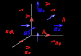
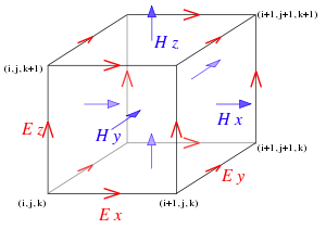 This description holds true for 1-D, 2-D, and 3-D FDTD techniques. When multiple dimensions are considered, calculating the numerical curl can become complicated. Kane Yee's seminal 1966 paper proposed spatially staggering the vector components of the E-field and H-field about rectangular unit cells of a Cartesian computational grid so that each E-field vector component is located midway between a pair of H-field vector components, and conversely. This scheme, now known as a Yee lattice, has proven to be very robust, and remains at the core of many current FDTD software constructs.
Furthermore, Yee proposed a leapfrog scheme for marching in time wherein the E-field and H-field updates are staggered so that E-field updates are conducted midway during each time-step between successive H-field updates, and conversely. On the plus side, this explicit time-stepping scheme avoids the need to solve simultaneous equations, and furthermore yields dissipation-free numerical wave propagation. On the minus side, this scheme mandates an upper bound on the time-step to ensure numerical stability. As a result, certain classes of simulations can require many thousands of time-steps for completion.
, or dielectric
. Any material can be used as long as the permeability
, permittivity
, and conductivity are specified.
Once the computational domain and the grid materials are established, a source is specified. The source can be an impinging plane wave, a current on a wire, or an applied electric field, depending on the application.
Since the E and H fields are determined directly, the output of the simulation is usually the E or H field at a point or a series of points within the computational domain. The simulation evolves the E and H fields forward in time.
Processing may be done on the E and H fields returned by the simulation. Data processing may also occur while the simulation is ongoing.
While the FDTD technique computes electromagnetic fields within a compact spatial region, scattered and/or radiated far fields can be obtained via near-to-far-field transformations.
FDTD is a versatile modeling technique used to solve Maxwell's equations. It is intuitive, so users can easily understand how to use it and know what to expect from a given model.
FDTD is a time-domain technique, and when a broadband pulse (such as a Gaussian pulse) is used as the source, then the response of the system over a wide range of frequencies can be obtained with a single simulation. This is useful in applications where resonant frequencies are not exactly known, or anytime that a broadband result is desired.
Since FDTD calculates the E and H fields everywhere in the computational domain as they evolve in time, it lends itself to providing animated displays of the electromagnetic field movement through the model. This type of display is useful in understanding what is going on in the model, and to help ensure that the model is working correctly.
The FDTD technique allows the user to specify the material at all points within the computational domain. A wide variety of linear and nonlinear dielectric and magnetic materials can be naturally and easily modeled.
FDTD allows the effects of apertures to be determined directly. Shielding effects can be found, and the fields both inside and outside a structure can be found directly or indirectly.
FDTD uses the E and H fields directly. Since most EMI/EMC modeling applications are interested in the E and H fields, it is convenient that no conversions must be made after the simulation has run to get these values.
There is no way to determine unique values for permittivity and permeability at a material interface.
Space and time steps must satisfy the CFL condition
.
FDTD finds the E/H fields directly everywhere in the computational domain. If the field values at some distance are desired, it is likely that this distance will force the computational domain to be excessively large. Far-field extensions are available for FDTD, but require some amount of postprocessing.
Since FDTD simulations calculate the E and H fields at all points within the computational domain, the computational domain must be finite to permit its residence in the computer memory. In many cases this is achieved by inserting artificial boundaries into the simulation space. Care must be taken to minimize errors introduced by such boundaries. There are a number of available highly effective absorbing boundary conditions (ABCs) to simulate an infinite unbounded computational domain. Most modern FDTD implementations instead use a special absorbing "material", called a perfectly matched layer
(PML) to implement absorbing boundaries.
Because FDTD is solved by propagating the fields forward in the time domain, the electromagnetic time response of the medium must be modeled explicitly. For an arbitrary response, this involves a computationally expensive time convolution, although in most cases the time response of the medium (or Dispersion (optics)
) can be adequately and simply modeled using either the recursive convolution (RC) technique, the auxiliary differential equation (ADE) technique, or the Z-transform technique. An alternative way of solving Maxwell's equations
that can treat arbitrary dispersion easily is the Pseudospectral Spatial-Domain method
(PSSD), which instead propagates the fields forward in space.
.
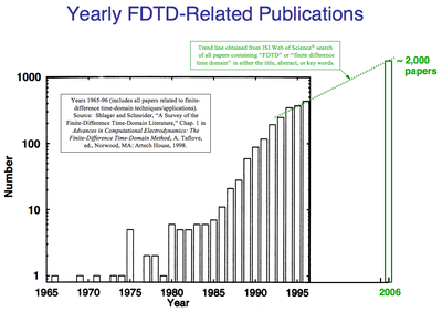 Interest in FDTD Maxwell’s equations solvers has increased nearly exponentially over the past 20 years. Increasingly, engineers and scientists in nontraditional electromagnetics-related areas such as photonics and nanotechnology have become aware of the power of FDTD techniques. As shown in the figure on the right, an estimated 2,000 FDTD-related publications appeared in the science and engineering literature in 2006, as opposed to fewer than 10 as recently as 1985. The current rate of growth (based upon a study of ISI Web of Science data) is approximately 5:1 over the period 1995 to 2006. Furthermore, the descriptor "finite difference time domain" has become widely used, having appeared in this exact form in 43,900 articles as of August 7, 2011, according to Google Scholar.
Notwithstanding both the general increase in academic publication throughput during the same period and the overall expansion of interest in all CEM
techniques,
there are seven primary reasons for the tremendous expansion of interest in FDTD computational solution approaches for Maxwell’s equations:
These factors combine to indicate that FDTD will likely remain one of the dominant computational electrodynamics techniques; and indeed may emerge as the dominant technique for mid-21st-century problems of surpassing volumetric complexity and/or multiphysics.
The following university-level textbooks provide a good general introduction to the FDTD method:
Time domain
Time domain is a term used to describe the analysis of mathematical functions, physical signals or time series of economic or environmental data, with respect to time. In the time domain, the signal or function's value is known for all real numbers, for the case of continuous time, or at various...
method, FDTD solutions can cover a wide frequency
Frequency
Frequency is the number of occurrences of a repeating event per unit time. It is also referred to as temporal frequency.The period is the duration of one cycle in a repeating event, so the period is the reciprocal of the frequency...
range with a single simulation
Computer simulation
A computer simulation, a computer model, or a computational model is a computer program, or network of computers, that attempts to simulate an abstract model of a particular system...
run, and treat nonlinear material properties in a natural way.
The FDTD method belongs in the general class of grid
Discretization
In mathematics, discretization concerns the process of transferring continuous models and equations into discrete counterparts. This process is usually carried out as a first step toward making them suitable for numerical evaluation and implementation on digital computers...
-based differential time-domain numerical modeling methods. The time-dependent Maxwell's equations
Maxwell's equations
Maxwell's equations are a set of partial differential equations that, together with the Lorentz force law, form the foundation of classical electrodynamics, classical optics, and electric circuits. These fields in turn underlie modern electrical and communications technologies.Maxwell's equations...
(in partial differential
Partial differential equation
In mathematics, partial differential equations are a type of differential equation, i.e., a relation involving an unknown function of several independent variables and their partial derivatives with respect to those variables...
form) are discretized using central-difference approximations to the space and time partial derivative
Partial derivative
In mathematics, a partial derivative of a function of several variables is its derivative with respect to one of those variables, with the others held constant...
s. The resulting finite-difference
Finite difference method
In mathematics, finite-difference methods are numerical methods for approximating the solutions to differential equations using finite difference equations to approximate derivatives.- Derivation from Taylor's polynomial :...
equations are solved in either software or hardware in a leapfrog
Leapfrog integration
Leapfrog integration is a simple method for numerically integrating differential equations of the form\ddot x=F,or equivalently of the form\dot v=F,\;\dot x \equiv v,particularly in the case of a dynamical system of classical mechanics...
manner: the electric field
Electric field
In physics, an electric field surrounds electrically charged particles and time-varying magnetic fields. The electric field depicts the force exerted on other electrically charged objects by the electrically charged particle the field is surrounding...
vector components in a volume of space are solved at a given instant in time; then the magnetic field
Magnetic field
A magnetic field is a mathematical description of the magnetic influence of electric currents and magnetic materials. The magnetic field at any given point is specified by both a direction and a magnitude ; as such it is a vector field.Technically, a magnetic field is a pseudo vector;...
vector components in the same spatial volume are solved at the next instant in time; and the process is repeated over and over again until the desired transient or steady-state electromagnetic field behavior is fully evolved.
The basic FDTD space grid and time-stepping algorithm trace back to a seminal 1966 paper by Kane Yee in IEEE Transactions on Antennas and Propagation. The descriptor "Finite-difference time-domain" and its corresponding "FDTD" acronym were originated by Allen Taflove
Allen Taflove
Allen Taflove is a full professor in the Department of Electrical Engineering and Computer Science of Northwestern's McCormick School of Engineering, since 1998...
in a 1980 paper in IEEE Transactions on Electromagnetic Compatibility.
Since about 1990, FDTD techniques have emerged as primary means to computationally model many scientific and engineering problems dealing with electromagnetic wave interactions with material structures. Current FDTD modeling applications range from near-DC
Direct current
Direct current is the unidirectional flow of electric charge. Direct current is produced by such sources as batteries, thermocouples, solar cells, and commutator-type electric machines of the dynamo type. Direct current may flow in a conductor such as a wire, but can also flow through...
(ultralow-frequency geophysics
Geophysics
Geophysics is the physics of the Earth and its environment in space; also the study of the Earth using quantitative physical methods. The term geophysics sometimes refers only to the geological applications: Earth's shape; its gravitational and magnetic fields; its internal structure and...
involving the entire Earth-ionosphere
Ionosphere
The ionosphere is a part of the upper atmosphere, comprising portions of the mesosphere, thermosphere and exosphere, distinguished because it is ionized by solar radiation. It plays an important part in atmospheric electricity and forms the inner edge of the magnetosphere...
waveguide) through microwaves (radar signature technology, antennas
Antenna (radio)
An antenna is an electrical device which converts electric currents into radio waves, and vice versa. It is usually used with a radio transmitter or radio receiver...
, wireless communications devices, digital interconnects, biomedical imaging/treatment) to visible light (photonic crystal
Photonic crystal
Photonic crystals are periodic optical nanostructures that are designed to affect the motion of photons in a similar way that periodicity of a semiconductor crystal affects the motion of electrons...
s, nanoplasmon
Plasmon
In physics, a plasmon is a quantum of plasma oscillation. The plasmon is a quasiparticle resulting from the quantization of plasma oscillations just as photons and phonons are quantizations of light and mechanical vibrations, respectively...
ics, soliton
Soliton
In mathematics and physics, a soliton is a self-reinforcing solitary wave that maintains its shape while it travels at constant speed. Solitons are caused by a cancellation of nonlinear and dispersive effects in the medium...
s, and biophotonics
Biophotonics
The term biophotonics denotes a combination of biology and photonics, with photonics being the science and technology of generation, manipulation, and detection of photons, quantum units of light. Photonics is related to electronics in that it is believed that photons will play a similar central...
). In 2006, an estimated 2,000 FDTD-related publications appeared in the science and engineering literature (see Popularity). At present (2008), there are at least 27 commercial/proprietary FDTD software vendors; 8 free-software/open-source
Open source
The term open source describes practices in production and development that promote access to the end product's source materials. Some consider open source a philosophy, others consider it a pragmatic methodology...
-software FDTD projects; and 2 freeware/closed-source FDTD projects, some not for commercial use (see External links).
Workings of the FDTD method
When Maxwell's differential equations are examined, it can be seen that the change in the E-field in time (the time derivative) is dependent on the change in the H-field across space (the curl). This results in the basic FDTD time-stepping relation that, at any point in space, the updated value of the E-field in time is dependent on the stored value of the E-field and the numerical curl of the local distribution of the H-field in space.The H-field is time-stepped in a similar manner. At any point in space, the updated value of the H-field in time is dependent on the stored value of the H-field and the numerical curl of the local distribution of the E-field in space. Iterating the E-field and H-field updates results in a marching-in-time process wherein sampled-data analogs of the continuous electromagnetic waves under consideration propagate in a numerical grid stored in the computer memory.
Furthermore, Yee proposed a leapfrog scheme for marching in time wherein the E-field and H-field updates are staggered so that E-field updates are conducted midway during each time-step between successive H-field updates, and conversely. On the plus side, this explicit time-stepping scheme avoids the need to solve simultaneous equations, and furthermore yields dissipation-free numerical wave propagation. On the minus side, this scheme mandates an upper bound on the time-step to ensure numerical stability. As a result, certain classes of simulations can require many thousands of time-steps for completion.
Using the FDTD method
To implement an FDTD solution of Maxwell's equations, a computational domain must first be established. The computational domain is simply the physical region over which the simulation will be performed. The E and H fields are determined at every point in space within that computational domain. The material of each cell within the computational domain must be specified. Typically, the material is either free-space (air), metalMetal
A metal , is an element, compound, or alloy that is a good conductor of both electricity and heat. Metals are usually malleable and shiny, that is they reflect most of incident light...
, or dielectric
Dielectric
A dielectric is an electrical insulator that can be polarized by an applied electric field. When a dielectric is placed in an electric field, electric charges do not flow through the material, as in a conductor, but only slightly shift from their average equilibrium positions causing dielectric...
. Any material can be used as long as the permeability
Permeability (electromagnetism)
In electromagnetism, permeability is the measure of the ability of a material to support the formation of a magnetic field within itself. In other words, it is the degree of magnetization that a material obtains in response to an applied magnetic field. Magnetic permeability is typically...
, permittivity
Permittivity
In electromagnetism, absolute permittivity is the measure of the resistance that is encountered when forming an electric field in a medium. In other words, permittivity is a measure of how an electric field affects, and is affected by, a dielectric medium. The permittivity of a medium describes how...
, and conductivity are specified.
Once the computational domain and the grid materials are established, a source is specified. The source can be an impinging plane wave, a current on a wire, or an applied electric field, depending on the application.
Since the E and H fields are determined directly, the output of the simulation is usually the E or H field at a point or a series of points within the computational domain. The simulation evolves the E and H fields forward in time.
Processing may be done on the E and H fields returned by the simulation. Data processing may also occur while the simulation is ongoing.
While the FDTD technique computes electromagnetic fields within a compact spatial region, scattered and/or radiated far fields can be obtained via near-to-far-field transformations.
Strengths of FDTD modeling
Every modeling technique has strengths and weaknesses, and the FDTD method is no different.FDTD is a versatile modeling technique used to solve Maxwell's equations. It is intuitive, so users can easily understand how to use it and know what to expect from a given model.
FDTD is a time-domain technique, and when a broadband pulse (such as a Gaussian pulse) is used as the source, then the response of the system over a wide range of frequencies can be obtained with a single simulation. This is useful in applications where resonant frequencies are not exactly known, or anytime that a broadband result is desired.
Since FDTD calculates the E and H fields everywhere in the computational domain as they evolve in time, it lends itself to providing animated displays of the electromagnetic field movement through the model. This type of display is useful in understanding what is going on in the model, and to help ensure that the model is working correctly.
The FDTD technique allows the user to specify the material at all points within the computational domain. A wide variety of linear and nonlinear dielectric and magnetic materials can be naturally and easily modeled.
FDTD allows the effects of apertures to be determined directly. Shielding effects can be found, and the fields both inside and outside a structure can be found directly or indirectly.
FDTD uses the E and H fields directly. Since most EMI/EMC modeling applications are interested in the E and H fields, it is convenient that no conversions must be made after the simulation has run to get these values.
Weaknesses of FDTD modeling
Since FDTD requires that the entire computational domain be gridded, and the grid spatial discretization must be sufficiently fine to resolve both the smallest electromagnetic wavelength and the smallest geometrical feature in the model, very large computational domains can be developed, which results in very long solution times. Models with long, thin features, (like wires) are difficult to model in FDTD because of the excessively large computational domain required.There is no way to determine unique values for permittivity and permeability at a material interface.
Space and time steps must satisfy the CFL condition
Courant–Friedrichs–Lewy condition
In mathematics, the Courant–Friedrichs–Lewy condition is a necessary condition for convergence while solving certain partial differential equations numerically by the method of finite differences. It arises when explicit time-marching schemes are used for the numerical solution...
.
FDTD finds the E/H fields directly everywhere in the computational domain. If the field values at some distance are desired, it is likely that this distance will force the computational domain to be excessively large. Far-field extensions are available for FDTD, but require some amount of postprocessing.
Since FDTD simulations calculate the E and H fields at all points within the computational domain, the computational domain must be finite to permit its residence in the computer memory. In many cases this is achieved by inserting artificial boundaries into the simulation space. Care must be taken to minimize errors introduced by such boundaries. There are a number of available highly effective absorbing boundary conditions (ABCs) to simulate an infinite unbounded computational domain. Most modern FDTD implementations instead use a special absorbing "material", called a perfectly matched layer
Perfectly matched layer
A perfectly matched layer is an artificial absorbing layer for wave equations, commonly used to truncate computational regions in numerical methods to simulate problems with open boundaries, especially in the FDTD and FEM methods...
(PML) to implement absorbing boundaries.
Because FDTD is solved by propagating the fields forward in the time domain, the electromagnetic time response of the medium must be modeled explicitly. For an arbitrary response, this involves a computationally expensive time convolution, although in most cases the time response of the medium (or Dispersion (optics)
Dispersion (optics)
In optics, dispersion is the phenomenon in which the phase velocity of a wave depends on its frequency, or alternatively when the group velocity depends on the frequency.Media having such a property are termed dispersive media...
) can be adequately and simply modeled using either the recursive convolution (RC) technique, the auxiliary differential equation (ADE) technique, or the Z-transform technique. An alternative way of solving Maxwell's equations
Maxwell's equations
Maxwell's equations are a set of partial differential equations that, together with the Lorentz force law, form the foundation of classical electrodynamics, classical optics, and electric circuits. These fields in turn underlie modern electrical and communications technologies.Maxwell's equations...
that can treat arbitrary dispersion easily is the Pseudospectral Spatial-Domain method
(PSSD), which instead propagates the fields forward in space.
Grid truncation techniques for open-region FDTD modeling problems
The most commonly used grid truncation techniques for open-region FDTD modeling problems are the Mur absorbing boundary condition (ABC), the Liao ABC, and various perfectly matched layer (PML) formulations. The Mur and Liao techniques are simpler than PML. However, PML (which is technically an absorbing region rather than a boundary condition per se) can provide orders-of-magnitude lower reflections. The PML concept was introduced by J.-P. Berenger in a seminal 1994 paper in the Journal of Computational Physics. Since 1994, Berenger's original split-field implementation has been modified and extended to the uniaxial PML (UPML), the convolutional PML (CPML), and the higher-order PML. The latter two PML formulations have increased ability to absorb evanescent waves, and therefore can in principle be placed closer to a simulated scattering or radiating structure than Berenger's original formulation.History of FDTD techniques and applications for Maxwell's equations
An appreciation of the basis, technical development, and possible future of FDTD numerical techniques for Maxwell’s equations can be developed by first considering their history. The following lists some of the key publications in this area, starting with Yee's seminal Paper #1 (1966), which has over 4,000 citations according to the ISI Web of ScienceWeb of Science
ISI Web of Knowledge is an academic citation indexing and search service, which is combined with web linking and provided by Thomson Reuters. Web of Knowledge coverage encompasses the sciences, social sciences, arts and humanities. It provides bibliographic content and the tools to access, analyze,...
.
| Partial chronology of FDTD techniques and applications for Maxwell's equations. | |
|---|---|
| year | event |
| 1966 | Yee described the basis of the FDTD numerical technique for solving Maxwell’s curl equations directly in the time domain on a space grid. |
| 1975 | Taflove and Brodwin reported the correct numerical stability criterion for Yee’s algorithm; the first sinusoidal steady-state FDTD solutions of two- and three-dimensional electromagnetic wave interactions with material structures; and the first bioelectromagnetics models. |
| 1977 | Holland and Kunz & Lee applied Yee’s algorithm to EMP problems. |
| 1980 | Taflove coined the FDTD acronym and published the first validated FDTD models of sinusoidal steady-state electromagnetic wave penetration into a three-dimensional metal cavity. |
| 1981 | Mur published the first numerically stable, second-order accurate, absorbing boundary condition (ABC) for Yee’s grid. |
| 1982–83 | Taflove and Umashankar developed the first FDTD electromagnetic wave scattering models computing sinusoidal steady-state near-fields, far-fields, and radar cross-section for two- and three-dimensional structures. |
| 1984 | Liao et al reported an improved ABC based upon space-time extrapolation of the field adjacent to the outer grid boundary. |
| 1985 | Gwarek introduced the lumped equivalent circuit formulation of FDTD. |
| 1986 | Choi and Hoefer published the first FDTD simulation of waveguide structures. |
| 1987–88 | Kriegsmann et al and Moore et al published the first articles on ABC theory in IEEE Transactions on Antennas and Propagation. |
| 1987–88, 1992 | Contour-path subcell techniques were introduced by Umashankar et al to permit FDTD modeling of thin wires and wire bundles, by Taflove et al to model penetration through cracks in conducting screens, and by Jurgens et al to conformally model the surface of a smoothly curved scatterer. |
| 1988 | Sullivan et al published the first 3-D FDTD model of sinusoidal steady-state electromagnetic wave absorption by a complete human body. |
| 1988 | FDTD modeling of microstrips was introduced by Zhang et al. |
| 1990–91 | FDTD modeling of frequency-dependent dielectric permittivity was introduced by Kashiwa and Fukai, Luebbers et al, and Joseph et al. |
| 1990–91 | FDTD modeling of antennas was introduced by Maloney et al, Katz et al, and Tirkas and Balanis. |
| 1990 | FDTD modeling of picosecond optoelectronic switches was introduced by Sano and Shibata, and El-Ghazaly et al. |
| 1992–94 | FDTD modeling of the propagation of optical pulses in nonlinear dispersive media was introduced, including the first temporal solitons in one dimension by Goorjian and Taflove; beam self-focusing by Ziolkowski and Judkins; the first temporal solitons in two dimensions by Joseph et al; and the first spatial solitons in two dimensions by Joseph and Taflove. |
| 1992 | FDTD modeling of lumped electronic circuit elements was introduced by Sui et al. |
| 1993 | Toland et al published the first FDTD models of gain devices (tunnel diodes and Gunn diodes) exciting cavities and antennas. |
| 1994 | Thomas et al introduced a Norton’s equivalent circuit for the FDTD space lattice, which permits the SPICE circuit analysis tool to implement accurate subgrid models of nonlinear electronic components or complete circuits embedded within the lattice. |
| 1994 | Berenger introduced the highly effective, perfectly matched layer (PML) ABC for two-dimensional FDTD grids, which was extended to three dimensions by Katz et al, and to dispersive waveguide terminations by Reuter et al. |
| 1995–96 | Sacks et al and Gedney introduced a physically realizable, uniaxial perfectly matched layer (UPML) ABC. |
| 1997 | Liu introduced the pseudospectral time-domain (PSTD) method, which permits extremely coarse spatial sampling of the electromagnetic field at the Nyquist limit. |
| 1997 | Ramahi introduced the complementary operators method (COM) to implement highly effective analytical ABCs. |
| 1998 | Maloney and Kesler introduced several novel means to analyze periodic structures in the FDTD space lattice. |
| 1998 | Nagra and York introduced a hybrid FDTD-quantum mechanics model of electromagnetic wave interactions with materials having electrons transitioning between multiple energy levels. |
| 1998 | Hagness et al introduced FDTD modeling of the detection of breast cancer using ultrawideband radar techniques. |
| 1999 | Schneider and Wagner introduced a comprehensive analysis of FDTD grid dispersion based upon complex wavenumbers. |
| 2000–01 | Zheng, Chen, and Zhang introduced the first three-dimensional alternating-direction implicit (ADI) FDTD algorithm with provable unconditional numerical stability. |
| 2000 | Roden and Gedney introduced the advanced convolutional PML (CPML) ABC. |
| 2000 | Rylander and Bondeson introduced a provably stable FDTD - finite-element time-domain hybrid technique. |
| 2002 | Hayakawa et al and Simpson and Taflove independently introduced FDTD modeling of the global Earth-ionosphere waveguide for extremely low-frequency geophysical phenomena. |
| 2003 | DeRaedt introduced the unconditionally stable, “one-step” FDTD technique. |
| 2008 | Ahmed, Chua, Li and Chen introduced the three-dimensional locally one dimensional (LOD)FDTD method and proved unconditional numerical stability. |
Popularity
Notwithstanding both the general increase in academic publication throughput during the same period and the overall expansion of interest in all CEM
Computational electromagnetics
Computational electromagnetics, computational electrodynamics or electromagnetic modeling is the process of modeling the interaction of electromagnetic fields with physical objects and the environment....
techniques,
there are seven primary reasons for the tremendous expansion of interest in FDTD computational solution approaches for Maxwell’s equations:
- FDTD uses no linear algebra. Being a fully explicit computation, FDTD avoids the difficulties with linear algebra that limit the size of frequency-domain integral-equation and finite-element electromagnetics models to generally fewer than 1e7 electromagnetic field unknowns. FDTD models with as many as 1e9 field unknowns have been run; there is no intrinsic upper bound to this number.
- FDTD is accurate and robust. The sources of error in FDTD calculations are well understood, and can be bounded to permit accurate models for a very large variety of electromagnetic wave interaction problems.
- FDTD treats impulsive behavior naturally. Being a time-domain technique, FDTD directly calculates the impulse response of an electromagnetic system. Therefore, a single FDTD simulation can provide either ultrawideband temporal waveforms or the sinusoidal steady-state response at any frequency within the excitation spectrum.
- FDTD treats nonlinear behavior naturally. Being a time-domain technique, FDTD directly calculates the nonlinear response of an electromagnetic system. This allows natural hybriding of FDTD with sets of auxiliary differential equations that describe nonlinearities from either the classical or semi-classical standpoint. An exciting research frontier here is the development of hybrid algorithms which join FDTD classical electrodynamics models with phenomena arising from quantum electrodynamics, especially vacuum fluctuations.
- FDTD is a systematic approach. With FDTD, specifying a new structure to be modeled is reduced to a problem of mesh generation rather than the potentially complex reformulation of an integral equation. For example, FDTD requires no calculation of structure-dependent Green functions.
- Parallel-processing computer architectures have come to dominate supercomputing. FDTD scales with high efficiency on parallel-processing CPU-based computers, and extremely well on recently developed GPU-based accelerator technology.
- Computer visualization capabilities are increasing rapidly. While this trend positively influences all numerical techniques, it is of particular advantage to FDTD methods, which generate time-marched arrays of field quantities suitable for use in color videos to illustrate the field dynamics.
These factors combine to indicate that FDTD will likely remain one of the dominant computational electrodynamics techniques; and indeed may emerge as the dominant technique for mid-21st-century problems of surpassing volumetric complexity and/or multiphysics.
See also
- Computational electromagneticsComputational electromagneticsComputational electromagnetics, computational electrodynamics or electromagnetic modeling is the process of modeling the interaction of electromagnetic fields with physical objects and the environment....
- Eigenmode expansionEigenmode expansionEigenmode Expansion is a computational electrodynamics modelling technique. It is also referred to as the mode matching technique or the Bidirectional Eigenmode Propagation method...
- Finite-difference frequency-domainFinite-difference frequency-domainThe finite-difference frequency-domain is a numerical solution for problems usually in electromagnetism, based on finite-difference approximations of the derivative operators in the differential equation being solved....
- Scattering Matrix MethodScattering Matrix MethodIn computational electromagnetics, the scattering-matrix method is a numerical method used to solve Maxwell's equations.-Principles:SMM can, for example, use cylinders to model dielectric/metal objects in the domain....
- Discrete dipole approximationDiscrete dipole approximationThe discrete dipole approximation is a method for computing scattering of radiation by particles of arbitrary shape and by periodic structures. Given a target of arbitrary geometry, one seeks to calculate its scattering and absorption properties...
Further reading
The following article in Nature Milestones: Photons illustrates the historical significance of the FDTD method as related to Maxwell's equations:The following university-level textbooks provide a good general introduction to the FDTD method:
External links
- Free softwareFree softwareFree software, software libre or libre software is software that can be used, studied, and modified without restriction, and which can be copied and redistributed in modified or unmodified form either without restriction, or with restrictions that only ensure that further recipients can also do...
/Open-source softwareOpen-source softwareOpen-source software is computer software that is available in source code form: the source code and certain other rights normally reserved for copyright holders are provided under a software license that permits users to study, change, improve and at times also to distribute the software.Open...
FDTD projects:- openEMS (Fully 3D Cartesian & Cylindrical graded mesh EC-FDTD Solver, written in C++, using a MatlabMATLABMATLAB is a numerical computing environment and fourth-generation programming language. Developed by MathWorks, MATLAB allows matrix manipulations, plotting of functions and data, implementation of algorithms, creation of user interfaces, and interfacing with programs written in other languages,...
/OctaveGNU OctaveGNU Octave is a high-level language, primarily intended for numerical computations. It provides a convenient command-line interface for solving linear and nonlinear problems numerically, and for performing other numerical experiments using a language that is mostly compatible with MATLAB...
-Interface) - pFDTD (3D C++ FDTD codes developed by Se-Heon Kim)
- JFDTD (2D/3D C++ FDTD codes developed for nanophotonics by Jeffrey M. McMahon)
- WOLFSIM (NCSU) (2-D)
- Meep (MITMassachusetts Institute of TechnologyThe Massachusetts Institute of Technology is a private research university located in Cambridge, Massachusetts. MIT has five schools and one college, containing a total of 32 academic departments, with a strong emphasis on scientific and technological education and research.Founded in 1861 in...
, 2D/3D/cylindrical parallel FDTD) - (Geo-) Radar FDTD
- bigboy (unmaintained, no release files. must get source from cvs)
- toyFDTD
- FDTD codes in C++ (developed by Zs. Szabó)
- FDTD code in Fortran 90
- FDTD code in C for 2D EM Wave simulation
- openEMS (Fully 3D Cartesian & Cylindrical graded mesh EC-FDTD Solver, written in C++, using a Matlab
- FreewareFreewareFreeware is computer software that is available for use at no cost or for an optional fee, but usually with one or more restricted usage rights. Freeware is in contrast to commercial software, which is typically sold for profit, but might be distributed for a business or commercial purpose in the...
/Closed source FDTD projects (some not for commercial use):- GprMax (Last updated on 12 May 2004 - unmaintained, no source code)
- EMTL (Electromagnetic Template Library) (Free С++ library for electromagnetic simulations. The current version implements mainly the FDTD).
- CommercialCommerceWhile business refers to the value-creating activities of an organization for profit, commerce means the whole system of an economy that constitutes an environment for business. The system includes legal, economic, political, social, cultural, and technological systems that are in operation in any...
/proprietaryProprietary softwareProprietary software is computer software licensed under exclusive legal right of the copyright holder. The licensee is given the right to use the software under certain conditions, while restricted from other uses, such as modification, further distribution, or reverse engineering.Complementary...
FDTD software vendors:- 2COMU
- Acceleware Inc.
- Agilent EEsof EDA EMPro(accessed 2009,April 13)
- Apollo Photonics
- Applied Simulation Technology
- Cray LC
- CST - Computer Simulation Technology
- Electro Magnetic Applications Inc.
- Emagware.com
- EM Explorer
- EM Photonics
- Empire
- EMS Plus
- ETHZ
- GdfidL
- Lumerical Solutions
- Nonlinear Control Strategies
- Optiwave
- Photon Design
- QuickWave
- Remcom XFdtd 7
- RM Associates
- Rsoft
- SPEAG - SEMCAD X
- Taflove-Hagness book software
- Tech-X Corporation
- Vector Fields
- Zeland