

Distributed parameter systems
Encyclopedia
A distributed parameter system (as opposed to a lumped parameter system) is a system
whose state space
is infinite-dimensional
. Such systems are therefore also known as infinite-dimensional systems. Typical examples are systems described by partial differential equation
s or by delay differential equation
s.
s and ∈ L(X),
  ∈ L(U, X),
  ∈ L(X, Y) and
  ∈ L(U, Y) the following equations determine a discrete-time linear time-invariant system:
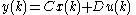
with (the state) a sequence with values in X,
  (the input or control) a sequence with values in U and
  (the output) a sequence with values in Y.
 ,
, .
.
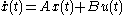
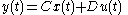
An added complication now however is that to include interesting physical examples such as partial differential equations and delay differential equations into this abstract framework, one is forced to consider unbounded operator
s. Usually A is assumed to generate a strongly continuous semigroup on the state space X. Assuming B, C and D to be bounded operators then already allows for the inclusion of many interesting physical examples, but the inclusion of many other interesting physical examples forces unboundedness of B and C as well.
 and
and  given by


fits into the abstract evolution equation framework described above as follows. The input space U and the output space Y are both chosen to be the set of complex numbers. The state space X is chosen to be L2(0, 1). The operator A is defined as
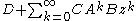
It can be shown that A generates a strongly continuous semigroup on X. The bounded operators B, C and D are defined as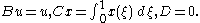


fits into the abstract evolution equation framework described above as follows. The input space U and the output space Y are both chosen to be the set of complex numbers. The state space X is chosen to be the product of the complex numbers with L2(−τ, 0). The operator A is defined as
It can be shown that A generates a strongly continuous semigroup on X. The bounded operators B, C and D are defined as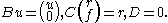
(discrete-time). Whereas in the finite-dimensional case the transfer function is a proper rational function, the infinite-dimensionality of the state space leads to irrational functions (which are however still holomorphic).
 and it is holomorphic in a disc centered at the origin. In case 1/z belongs to the resolvent set of A (which is the case on a possibly smaller disc centered at the origin) the transfer function equals
 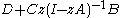 . An interesting fact is that any function that is holomorphic in zero is the transfer function of some discrete-time system.
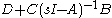 for s with real part larger than the exponential growth bound of the semigroup generated by A. In more general situations this formula as it stands may not even make sense, but an appropriate generalization of this formula still holds.
To obtain an easy expression for the transfer function it is often better to take the Laplace transform in the given differential equation than to use the state space formulas as illustrated below on the examples given above.
 equal to zero and denoting Laplace transforms with respect to t by capital letters we obtain from the partial differential equation given above
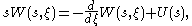

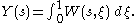
This is an inhomogeneous linear differential equation with as the variable, s as a parameter and initial condition zero. The solution is
 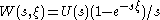 . Substituting this in the equation for Y and integrating gives
  so that the transfer function is
  .
.
 .
.
which for the finite-dimensional case collapse to the one usual notion of controllability. The three most important controllability concepts are:
 which map the set of all U valued sequences into X and are given by
 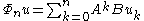 . The interpretation is that
  is the state that is reached by applying the input sequence u when the initial condition is zero. The system is called
 given by
 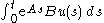 plays the role that
  plays in discrete-time. However, the space of control functions on which this operator acts now influences the definition. The usual choice is L2(0, ∞;U), the space of (equivalence classes of) U-valued square integrable functions on the interval (0, ∞), but other choices such as L1(0, ∞;U) are possible. The different controllability notions can be defined once the domain of
  is chosen. The system is called
is the dual notion of controllability. In the infinite-dimensional case there are several different notions of observability which in the finite-dimensional case coincide. The three most important ones are:
 which map X into the space of all Y valued sequences and are given by
 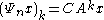 if k ≤ n and zero if k > n. The interpretation is that
  is the truncated output with initial condition x and control zero. The system is called
 given by
 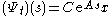 for s∈[0,t] and zero for s>t plays the role that
  plays in discrete-time. However, the space of functions to which this operator maps now influences the definition. The usual choice is L2(0, ∞, Y), the space of (equivalence classes of) Y-valued square integrable functions on the interval (0,∞), but other choices such as L1(0, ∞, Y) are possible. The different observability notions can be defined once the co-domain of
  is chosen. The system is called
 and the co-domain of
  the usual L2 choice is made). The correspondence under duality of the different concepts is:
System
System is a set of interacting or interdependent components forming an integrated whole....
whose state space
State space (controls)
In control engineering, a state space representation is a mathematical model of a physical system as a set of input, output and state variables related by first-order differential equations...
is infinite-dimensional
Dimension (vector space)
In mathematics, the dimension of a vector space V is the cardinality of a basis of V. It is sometimes called Hamel dimension or algebraic dimension to distinguish it from other types of dimension...
. Such systems are therefore also known as infinite-dimensional systems. Typical examples are systems described by partial differential equation
Partial differential equation
In mathematics, partial differential equations are a type of differential equation, i.e., a relation involving an unknown function of several independent variables and their partial derivatives with respect to those variables...
s or by delay differential equation
Delay differential equation
In mathematics, delay differential equations are a type of differential equation in which the derivative of the unknown function at a certain time is given in terms of the values of the function at previous times....
s.
Discrete-time
With U, X and Y Hilbert spaceHilbert space
The mathematical concept of a Hilbert space, named after David Hilbert, generalizes the notion of Euclidean space. It extends the methods of vector algebra and calculus from the two-dimensional Euclidean plane and three-dimensional space to spaces with any finite or infinite number of dimensions...
s and
∈ L(X), ∈ L(U, X), ∈ L(X, Y) and ∈ L(U, Y) the following equations determine a discrete-time linear time-invariant system:with
(the state) a sequence with values in X, (the input or control) a sequence with values in U and (the output) a sequence with values in Y.Continuous-time
The continuous-time case is similar to the discrete-time case but now one considers differential equations instead of difference equations:,.An added complication now however is that to include interesting physical examples such as partial differential equations and delay differential equations into this abstract framework, one is forced to consider unbounded operator
Unbounded operator
In mathematics, more specifically functional analysis and operator theory, the notion of unbounded operator provides an abstract framework for dealing with differential operators, unbounded observables in quantum mechanics, and other cases....
s. Usually A is assumed to generate a strongly continuous semigroup on the state space X. Assuming B, C and D to be bounded operators then already allows for the inclusion of many interesting physical examples, but the inclusion of many other interesting physical examples forces unboundedness of B and C as well.
Example: a partial differential equation
The partial differential equation with and given byfits into the abstract evolution equation framework described above as follows. The input space U and the output space Y are both chosen to be the set of complex numbers. The state space X is chosen to be L2(0, 1). The operator A is defined as
It can be shown that A generates a strongly continuous semigroup on X. The bounded operators B, C and D are defined as
Example: a delay differential equation
The delay differential equationfits into the abstract evolution equation framework described above as follows. The input space U and the output space Y are both chosen to be the set of complex numbers. The state space X is chosen to be the product of the complex numbers with L2(−τ, 0). The operator A is defined as
It can be shown that A generates a strongly continuous semigroup on X. The bounded operators B, C and D are defined as
Transfer functions
As in the finite-dimensional case the transfer function is defined through the Laplace transform (continuous-time) or Z-transformZ-transform
In mathematics and signal processing, the Z-transform converts a discrete time-domain signal, which is a sequence of real or complex numbers, into a complex frequency-domain representation....
(discrete-time). Whereas in the finite-dimensional case the transfer function is a proper rational function, the infinite-dimensionality of the state space leads to irrational functions (which are however still holomorphic).
Discrete-time
In discrete-time the transfer function is given in terms of the state space parameters by and it is holomorphic in a disc centered at the origin. In case 1/z belongs to the resolvent set of A (which is the case on a possibly smaller disc centered at the origin) the transfer function equals . An interesting fact is that any function that is holomorphic in zero is the transfer function of some discrete-time system.Continuous-time
If A generates a strongly continuous semigroup and B, C and D are bounded operators, then the transfer function is given in terms of the state space parameters by for s with real part larger than the exponential growth bound of the semigroup generated by A. In more general situations this formula as it stands may not even make sense, but an appropriate generalization of this formula still holds.To obtain an easy expression for the transfer function it is often better to take the Laplace transform in the given differential equation than to use the state space formulas as illustrated below on the examples given above.
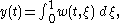
Transfer function for the partial differential equation example
Setting the initial condition equal to zero and denoting Laplace transforms with respect to t by capital letters we obtain from the partial differential equation given aboveThis is an inhomogeneous linear differential equation with
as the variable, s as a parameter and initial condition zero. The solution is . Substituting this in the equation for Y and integrating gives so that the transfer function is .Transfer function for the delay differential equation example
Proceeding similarly as for the partial differential equation example, the transfer function for the delay equation example is.Controllability
In the infinite-dimensional case there are several non-equivalent definitions of controllabilityControllability
Controllability is an important property of a control system, and the controllability property plays a crucial role in many control problems, such as stabilization of unstable systems by feedback, or optimal control....
which for the finite-dimensional case collapse to the one usual notion of controllability. The three most important controllability concepts are:
- Exact controllability,
- Approximate controllability,
- Null controllability.
Controllability in discrete-time
An important role is played by the maps which map the set of all U valued sequences into X and are given by . The interpretation is that is the state that is reached by applying the input sequence u when the initial condition is zero. The system is called
- exactly controllable in time n if the range of
 equals X,
 - approximately controllable in time n if the range of
 is dense in X,
 - null controllable in time n if the range of
 includes the range of An.
Controllability in continuous-time
In controllability of continuous-time systems the map given by plays the role that plays in discrete-time. However, the space of control functions on which this operator acts now influences the definition. The usual choice is L2(0, ∞;U), the space of (equivalence classes of) U-valued square integrable functions on the interval (0, ∞), but other choices such as L1(0, ∞;U) are possible. The different controllability notions can be defined once the domain of is chosen. The system is called
- exactly controllable in time t if the range of
 equals X,
 - approximately controllable in time t if the range of
 is dense in X,
 - null controllable in time t if the range of
 includes the range of
  .
.
Observability
As in the finite-dimensional case, observabilityObservability
Observability, in control theory, is a measure for how well internal states of a system can be inferred by knowledge of its external outputs. The observability and controllability of a system are mathematical duals. The concept of observability was introduced by American-Hungarian scientist Rudolf E...
is the dual notion of controllability. In the infinite-dimensional case there are several different notions of observability which in the finite-dimensional case coincide. The three most important ones are:
- Exact observability (also known as continuous observability),
- Approximate observability,
- Final state observability.
Observability in discrete-time
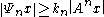
An important role is played by the maps which map X into the space of all Y valued sequences and are given by if k ≤ n and zero if k > n. The interpretation is that is the truncated output with initial condition x and control zero. The system is called
- exactly observable in time n if there exists a kn > 0 such that
 for all x ∈ X,
 - approximately observable in time n if
 is injective,
 - final state observable in time n if there exists a kn > 0 such that
 for all x ∈ X.
Observability in continuous-time
In observability of continuous-time systems the map given by for s∈[0,t] and zero for s>t plays the role that plays in discrete-time. However, the space of functions to which this operator maps now influences the definition. The usual choice is L2(0, ∞, Y), the space of (equivalence classes of) Y-valued square integrable functions on the interval (0,∞), but other choices such as L1(0, ∞, Y) are possible. The different observability notions can be defined once the co-domain of is chosen. The system is called
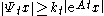
- exactly observable in time t if there exists a kt > 0 such that
 for all x ∈ X,
 - approximately observable in time t if
 is injective,
 - final state observable in time t if there exists a kt > 0 such that
 for all x ∈ X.
Duality between controllability and observability
As in the finite-dimensional case, controllability and observability are dual concepts (at least when for the domain of and the co-domain of the usual L2 choice is made). The correspondence under duality of the different concepts is:
- Exact controllability ↔ Exact observability,
- Approximate controllability ↔ Approximate observability,
- Null controllability ↔ Final state observability.