
Dijkstra's algorithm
Encyclopedia
Dijkstra's algorithm, conceived by Dutch computer scientist
Edsger Dijkstra
in 1956 and published in 1959, is a graph search algorithm that solves the single-source shortest path problem
for a graph
with nonnegative edge path costs, producing a shortest path tree
. This algorithm is often used in routing
and as a subroutine in other graph algorithms.
For a given source vertex
(node) in the graph, the algorithm finds the path with lowest cost (i.e. the shortest path) between that vertex and every other vertex. It can also be used for finding costs of shortest paths from a single vertex to a single destination vertex by stopping the algorithm once the shortest path to the destination vertex has been determined. For example, if the vertices of the graph represent cities and edge path costs represent driving distances between pairs of cities connected by a direct road, Dijkstra's algorithm can be used to find the shortest route between one city and all other cities. As a result, the shortest path first is widely used in network routing protocol
s, most notably IS-IS
and OSPF (Open Shortest Path First).
Dijkstra's original algorithm does not use a min-priority queue and runs in O(|V|2). The idea of this algorithm is also given in . The common implementation based on a min-priority queue implemented by a Fibonacci heap
and running in O(|E| + |V| log |V|) is due to . This is asymptotically
the fastest known single-source shortest-path algorithm for arbitrary directed graphs with unbounded nonnegative weights. (For an overview of earlier shortest path algorithms and later improvements and adaptations, see: Single-source shortest-paths algorithms for directed graphs with nonnegative weights.)
Suppose you want to find the shortest path between two intersections
on a city map, a starting point and a destination. The order is conceptually simple: to start, mark the distance to every intersection on the map with infinity. This is done not to imply there is an infinite distance, but to note that that intersection has not yet been visited. (Some variants of this method simply leave the intersection unlabeled.) Now, at each iteration, select a current intersection. For the first iteration the current intersection will be the starting point and the distance to it (the intersection's label) will be zero. For subsequent iterations (after the first) the current intersection will be the closest unvisited intersection to the starting point—this will be easy to find.
From the current intersection, update the distance to every unvisited intersection that is directly connected to it. This is done by determining the sum of the distance between an unvisited intersection and the value of the current intersection, and relabeling
the unvisited intersection with this value if it is less than its current value. In effect, the intersection is relabeled if the path to it through the current intersection is shorter than the previously known paths. To facilitate shortest path identification, in pencil, mark the road with an arrow pointing to the relabeled intersection if you label/relabel it, and erase all others pointing to it. After you have updated the distances to each neighboring intersection
, mark the current intersection as visited and select the unvisited intersection with lowest distance (from the starting point) -- or lowest label—as the current intersection. Nodes marked as visited are labeled with the shortest path from the starting point to it and will not be revisited or returned to.
Continue this process of updating the neighboring intersections with the shortest distances, then marking the current intersection as visited and moving onto the closest unvisited intersection until you have marked the destination as visited. Once you have marked the destination as visited (as is the case with any visited intersection) you have determined the shortest path to it, from the starting point, and can trace your way back, following the arrows in reverse.
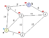
In the accompanying animated graphic, the starting and destination intersections are colored in light pink and blue and labelled a and b respectively. The visited intersections are colored in red, and the current intersection in a pale blue.
Of note is the fact that this algorithm makes no attempt to direct "exploration" towards the destination as one might expect. Rather, the sole consideration in determining the next "current" intersection is its distance from the starting point. In some sense, this algorithm "expands outward" from the starting point, iteratively considering every node that is closer in terms of shortest path distance until it reaches the destination. When understood in this way, it is clear how the algorithm necessarily finds the shortest path, however it may also reveal one of the algorithm's weaknesses: its relative slowness in some topologies.
1 function Dijkstra(Graph, source):
2 for each vertex v in Graph: // Initializations
3 dist[v] := infinity ; // Unknown distance function from source to v
4 previous[v] := undefined ; // Previous node in optimal path from source
5 end for ;
6 dist[source] := 0 ; // Distance from source to source
7 Q := the set of all nodes in Graph ; // All nodes in the graph are unoptimized - thus are in Q
8 while Q is not empty: // The main loop
9 u := vertex in Q with smallest distance in dist[] ;
10 if dist[u] = infinity:
11 break ; // all remaining vertices are inaccessible from source
12 end if ;
13 remove u from Q ;
14 for each neighbor v of u: // where v has not yet been removed from Q.
15 alt := dist[u] + dist_between(u, v) ;
16 if alt < dist[v]: // Relax (u,v,a)
17 dist[v] := alt ;
18 previous[v] := u ;
19 decrease-key v in Q; // Reorder v in the Queue
20 end if ;
21 end for ;
22 end while ;
23 return dist[] ;
24 end Dijkstra.
If we are only interested in a shortest path between vertices
Now we can read the shortest path from
1 S := empty sequence
2 u := target
3 while previous[u] is defined:
4 insert u at the beginning of S
5 u := previous[u]
6 end while ;
Now sequence
A more general problem would be to find all the shortest paths between
 and vertices
  can be expressed as a function of
  and
and  using Big-O notation.
For any implementation of vertex set the running time is
  , where
  and
and  are times needed to perform decrease key and extract minimum operations in set
  , respectively.
The simplest implementation of the Dijkstra's algorithm stores vertices of set in an ordinary linked list or array, and extract minimum from
  is simply a linear search through all vertices in
  . In this case, the running time is
  .
.
For sparse graphs, that is, graphs with far fewer than edges, Dijkstra's algorithm can be implemented more efficiently by storing the graph in the form of adjacency list
s and using a binary heap
, pairing heap
, or Fibonacci heap
as a priority queue
to implement extracting minimum efficiently. With a binary heap, the algorithm requires time (which is dominated by O( | E | log | V | ), assuming the graph is connected). To avoid O(|V|) look-up in decrease-key step on a vanilla binary heap, it is necessary to maintain a supplementary index mapping each vertex to the heap's index (and keep it up to date as priority queue
  changes), making it take only
  time instead. The Fibonacci heap
improves this to .
.
Note that for Directed acyclic graph
s, it is possible to find shortest paths from a given starting vertex in linear time, by processing the vertices in a topological order, and calculating the path length for each vertex to be the minimum length obtained via any of its incoming edges.
Dijkstra's algorithm is usually the working principle behind link-state routing protocol
s, OSPF and IS-IS
being the most common ones.
Unlike Dijkstra's algorithm, the Bellman-Ford algorithm
can be used on graphs with negative edge weights, as long as the graph contains no negative cycle reachable from the source vertex s. (The presence of such cycles means there is no shortest path, since the total weight becomes lower each time the cycle is traversed.)
The A* algorithm is a generalization of Dijkstra's algorithm that cuts down on the size of the subgraph that must be explored, if additional information is available that provides a lower bound on the "distance" to the target. This approach can be viewed from the perspective of linear programming
: there is a natural linear program for computing shortest paths, and solutions to its dual linear program are feasible if and only if they form a consistent heuristic
(speaking roughly, since the sign conventions differ from place to place in the literature). This feasible dual / consistent heuristic defines a nonnegative reduced cost
and A* is essentially running Dijkstra's algorithm with these reduced costs. If the dual satisfies the weaker condition of admissibility, then A* is instead more akin to the Bellman-Ford algorithm.
The process that underlies Dijkstra's algorithm is similar to the greedy process used in Prim's algorithm
. Prim's purpose is to find a minimum spanning tree
that connects all nodes in the graph; Dijkstra is concerned with only two nodes. Prim's does not evaluate the total weight of the path from the starting node, only the individual path.
point of view, Dijkstra's algorithm is a successive approximation scheme that solves the dynamic programming functional equation for the shortest path problem by the Reaching method.
In fact, Dijkstra's explanation of the logic behind the algorithm, namely
is a paraphrasing of Bellman's
famous Principle of Optimality in the context of the shortest path problem.
Computer scientist
A computer scientist is a scientist who has acquired knowledge of computer science, the study of the theoretical foundations of information and computation and their application in computer systems....
Edsger Dijkstra
Edsger Dijkstra
Edsger Wybe Dijkstra ; ) was a Dutch computer scientist. He received the 1972 Turing Award for fundamental contributions to developing programming languages, and was the Schlumberger Centennial Chair of Computer Sciences at The University of Texas at Austin from 1984 until 2000.Shortly before his...
in 1956 and published in 1959, is a graph search algorithm that solves the single-source shortest path problem
Shortest path problem
In graph theory, the shortest path problem is the problem of finding a path between two vertices in a graph such that the sum of the weights of its constituent edges is minimized...
for a graph
Graph (mathematics)
In mathematics, a graph is an abstract representation of a set of objects where some pairs of the objects are connected by links. The interconnected objects are represented by mathematical abstractions called vertices, and the links that connect some pairs of vertices are called edges...
with nonnegative edge path costs, producing a shortest path tree
Shortest path tree
A shortest path tree, in graph theory, is a subgraph of a given graph constructed so that the distance between a selected root node and all other nodes is minimal. It is a tree because if there are two paths between the root node and some vertex v A shortest path tree, in graph theory, is a...
. This algorithm is often used in routing
Routing
Routing is the process of selecting paths in a network along which to send network traffic. Routing is performed for many kinds of networks, including the telephone network , electronic data networks , and transportation networks...
and as a subroutine in other graph algorithms.
For a given source vertex
Vertex (graph theory)
In graph theory, a vertex or node is the fundamental unit out of which graphs are formed: an undirected graph consists of a set of vertices and a set of edges , while a directed graph consists of a set of vertices and a set of arcs...
(node) in the graph, the algorithm finds the path with lowest cost (i.e. the shortest path) between that vertex and every other vertex. It can also be used for finding costs of shortest paths from a single vertex to a single destination vertex by stopping the algorithm once the shortest path to the destination vertex has been determined. For example, if the vertices of the graph represent cities and edge path costs represent driving distances between pairs of cities connected by a direct road, Dijkstra's algorithm can be used to find the shortest route between one city and all other cities. As a result, the shortest path first is widely used in network routing protocol
Routing protocol
A routing protocol is a protocol that specifies how routers communicate with each other, disseminating information that enables them to select routes between any two nodes on a computer network, the choice of the route being done by routing algorithms. Each router has a priori knowledge only of...
s, most notably IS-IS
IS-IS
Intermediate System To Intermediate System , is a routing protocol designed to move information efficiently within a computer network, a group of physically connected computers or similar devices....
and OSPF (Open Shortest Path First).
Dijkstra's original algorithm does not use a min-priority queue and runs in O(|V|2). The idea of this algorithm is also given in . The common implementation based on a min-priority queue implemented by a Fibonacci heap
Fibonacci heap
In computer science, a Fibonacci heap is a heap data structure consisting of a collection of trees. It has a better amortized running time than a binomial heap. Fibonacci heaps were developed by Michael L. Fredman and Robert E. Tarjan in 1984 and first published in a scientific journal in 1987...
and running in O(|E| + |V| log |V|) is due to . This is asymptotically
Asymptotic computational complexity
In computational complexity theory, asymptotic computational complexity is the usage of the asymptotic analysis for the estimation of computational complexity of algorithms and computational problems, commonly associated with the usage of the big O notation....
the fastest known single-source shortest-path algorithm for arbitrary directed graphs with unbounded nonnegative weights. (For an overview of earlier shortest path algorithms and later improvements and adaptations, see: Single-source shortest-paths algorithms for directed graphs with nonnegative weights.)
Algorithm
Let the node at which we are starting be called the initial node. Let the distance of node Y be the distance from the initial node to Y. Dijkstra's algorithm will assign some initial distance values and will try to improve them step by step.- Assign to every node a tentative distance value: set it to zero for our initial node and to infinity for all other nodes.
- Mark all nodes unvisited. Set the initial node as current. Create a set of the unvisited nodes called the unvisited set consisting of all the nodes except the initial node.
- For the current node, consider all of its unvisited neighbors and calculate their tentative distances. For example, if the current node A is marked with a distance of 6, and the edge connecting it with a neighbor B has length 2, then the distance to B (through A) will be 6+2=8. If this distance is less than the previously recorded distance, then overwrite that distance. Even though a neighbor has been examined, it is not marked as visited at this time, and it remains in the unvisited set.
- When we are done considering all of the neighbors of the current node, mark the current node as visited and remove it from the unvisited set. A visited node will never be checked again; its distance recorded now is final and minimal.
- If the unvisited set is empty, then stop. The algorithm has finished.
- Set the unvisited node marked with the smallest tentative distance as the next "current node" and go back to step 3.
Description
- Note: For ease of understanding, this discussion uses the terms intersection, road and map — however, formally these terms are vertex, edge and graph, respectively.
Suppose you want to find the shortest path between two intersections
Intersection (road)
An intersection is a road junction where two or more roads either meet or cross at grade . An intersection may be 3-way - a T junction or fork, 4-way - a crossroads, or 5-way or more...
on a city map, a starting point and a destination. The order is conceptually simple: to start, mark the distance to every intersection on the map with infinity. This is done not to imply there is an infinite distance, but to note that that intersection has not yet been visited. (Some variants of this method simply leave the intersection unlabeled.) Now, at each iteration, select a current intersection. For the first iteration the current intersection will be the starting point and the distance to it (the intersection's label) will be zero. For subsequent iterations (after the first) the current intersection will be the closest unvisited intersection to the starting point—this will be easy to find.
From the current intersection, update the distance to every unvisited intersection that is directly connected to it. This is done by determining the sum of the distance between an unvisited intersection and the value of the current intersection, and relabeling
Graph labeling
In the mathematical discipline of graph theory, a graph labeling is the assignment of labels, traditionally represented by integers, to the edges or vertices, or both, of a graph....
the unvisited intersection with this value if it is less than its current value. In effect, the intersection is relabeled if the path to it through the current intersection is shorter than the previously known paths. To facilitate shortest path identification, in pencil, mark the road with an arrow pointing to the relabeled intersection if you label/relabel it, and erase all others pointing to it. After you have updated the distances to each neighboring intersection
Neighbourhood (graph theory)
In graph theory, an adjacent vertex of a vertex v in a graph is a vertex that is connected to v by an edge. The neighbourhood of a vertex v in a graph G is the induced subgraph of G consisting of all vertices adjacent to v and all edges connecting two such vertices. For example, the image shows a...
, mark the current intersection as visited and select the unvisited intersection with lowest distance (from the starting point) -- or lowest label—as the current intersection. Nodes marked as visited are labeled with the shortest path from the starting point to it and will not be revisited or returned to.
Continue this process of updating the neighboring intersections with the shortest distances, then marking the current intersection as visited and moving onto the closest unvisited intersection until you have marked the destination as visited. Once you have marked the destination as visited (as is the case with any visited intersection) you have determined the shortest path to it, from the starting point, and can trace your way back, following the arrows in reverse.
In the accompanying animated graphic, the starting and destination intersections are colored in light pink and blue and labelled a and b respectively. The visited intersections are colored in red, and the current intersection in a pale blue.
Of note is the fact that this algorithm makes no attempt to direct "exploration" towards the destination as one might expect. Rather, the sole consideration in determining the next "current" intersection is its distance from the starting point. In some sense, this algorithm "expands outward" from the starting point, iteratively considering every node that is closer in terms of shortest path distance until it reaches the destination. When understood in this way, it is clear how the algorithm necessarily finds the shortest path, however it may also reveal one of the algorithm's weaknesses: its relative slowness in some topologies.
Pseudocode
In the following algorithm, the codeu := vertex in Q with smallest dist[], searches for the vertex u in the vertex set Q that has the least dist[u] value. That vertex is removed from the set Q and returned to the user. dist_between(u, v) calculates the length between the two neighbor-nodes u and v. The variable alt on line 15 is the length of the path from the root node to the neighbor node v if it were to go through u. If this path is shorter than the current shortest path recorded for v, that current path is replaced with this alt path. The previous array is populated with a pointer to the "next-hop" node on the source graph to get the shortest route to the source.1 function Dijkstra(Graph, source):
2 for each vertex v in Graph: // Initializations
3 dist[v] := infinity ; // Unknown distance function from source to v
4 previous[v] := undefined ; // Previous node in optimal path from source
5 end for ;
6 dist[source] := 0 ; // Distance from source to source
7 Q := the set of all nodes in Graph ; // All nodes in the graph are unoptimized - thus are in Q
8 while Q is not empty: // The main loop
9 u := vertex in Q with smallest distance in dist[] ;
10 if dist[u] = infinity:
11 break ; // all remaining vertices are inaccessible from source
12 end if ;
13 remove u from Q ;
14 for each neighbor v of u: // where v has not yet been removed from Q.
15 alt := dist[u] + dist_between(u, v) ;
16 if alt < dist[v]: // Relax (u,v,a)
17 dist[v] := alt ;
18 previous[v] := u ;
19 decrease-key v in Q; // Reorder v in the Queue
20 end if ;
21 end for ;
22 end while ;
23 return dist[] ;
24 end Dijkstra.
If we are only interested in a shortest path between vertices
source and target, we can terminate the search at line 13 if u = target.Now we can read the shortest path from
source to target by iteration:1 S := empty sequence
2 u := target
3 while previous[u] is defined:
4 insert u at the beginning of S
5 u := previous[u]
6 end while ;
Now sequence
S is the list of vertices constituting one of the shortest paths from source to target, or the empty sequence if no path exists.A more general problem would be to find all the shortest paths between
source and target (there might be several different ones of the same length). Then instead of storing only a single node in each entry of previous[] we would store all nodes satisfying the relaxation condition. For example, if both r and source connect to target and both of them lie on different shortest paths through target (because the edge cost is the same in both cases), then we would add both r and source to previous[target]. When the algorithm completes, previous[] data structure will actually describe a graph that is a subset of the original graph with some edges removed. Its key property will be that if the algorithm was run with some starting node, then every path from that node to any other node in the new graph will be the shortest path between those nodes in the original graph, and all paths of that length from the original graph will be present in the new graph. Then to actually find all these short paths between two given nodes we would use a path finding algorithm on the new graph, such as depth-first search.Running time
An upper bound of the running time of Dijkstra's algorithm on a graph with edges and vertices can be expressed as a function of and using Big-O notation.For any implementation of vertex set
the running time is , where and are times needed to perform decrease key and extract minimum operations in set , respectively.The simplest implementation of the Dijkstra's algorithm stores vertices of set
in an ordinary linked list or array, and extract minimum from is simply a linear search through all vertices in . In this case, the running time is .For sparse graphs, that is, graphs with far fewer than
edges, Dijkstra's algorithm can be implemented more efficiently by storing the graph in the form of adjacency listAdjacency list
In graph theory, an adjacency list is the representation of all edges or arcs in a graph as a list.If the graph is undirected, every entry is a set of two nodes containing the two ends of the corresponding edge; if it is directed, every entry is a tuple of two nodes, one denoting the source node...
s and using a binary heap
Binary heap
A binary heap is a heap data structure created using a binary tree. It can be seen as a binary tree with two additional constraints:*The shape property: the tree is a complete binary tree; that is, all levels of the tree, except possibly the last one are fully filled, and, if the last level of...
, pairing heap
Pairing heap
A pairing heaps is a type of heap data structure with relatively simple implementation and excellent practical amortized performance. However, it has proven very difficult to determine the precise asymptotic running time of pairing heaps....
, or Fibonacci heap
Fibonacci heap
In computer science, a Fibonacci heap is a heap data structure consisting of a collection of trees. It has a better amortized running time than a binomial heap. Fibonacci heaps were developed by Michael L. Fredman and Robert E. Tarjan in 1984 and first published in a scientific journal in 1987...
as a priority queue
Priority queue
A priority queue is an abstract data type in computer programming.It is exactly like a regular queue or stack data structure, but additionally, each element is associated with a "priority"....
to implement extracting minimum efficiently. With a binary heap, the algorithm requires
time (which is dominated by O( | E | log | V | ), assuming the graph is connected). To avoid O(|V|) look-up in decrease-key step on a vanilla binary heap, it is necessary to maintain a supplementary index mapping each vertex to the heap's index (and keep it up to date as priority queue changes), making it take only time instead. The Fibonacci heapFibonacci heap
In computer science, a Fibonacci heap is a heap data structure consisting of a collection of trees. It has a better amortized running time than a binomial heap. Fibonacci heaps were developed by Michael L. Fredman and Robert E. Tarjan in 1984 and first published in a scientific journal in 1987...
improves this to
.Note that for Directed acyclic graph
Directed acyclic graph
In mathematics and computer science, a directed acyclic graph , is a directed graph with no directed cycles. That is, it is formed by a collection of vertices and directed edges, each edge connecting one vertex to another, such that there is no way to start at some vertex v and follow a sequence of...
s, it is possible to find shortest paths from a given starting vertex in linear time, by processing the vertices in a topological order, and calculating the path length for each vertex to be the minimum length obtained via any of its incoming edges.
Related problems and algorithms
The functionality of Dijkstra's original algorithm can be extended with a variety of modifications. For example, sometimes it is desirable to present solutions which are less than mathematically optimal. To obtain a ranked list of less-than-optimal solutions, the optimal solution is first calculated. A single edge appearing in the optimal solution is removed from the graph, and the optimum solution to this new graph is calculated. Each edge of the original solution is suppressed in turn and a new shortest-path calculated. The secondary solutions are then ranked and presented after the first optimal solution.Dijkstra's algorithm is usually the working principle behind link-state routing protocol
Link-state routing protocol
A link-state routing protocol is one of the two main classes of routing protocols used in packet switching networks for computer communications . Examples of link-state routing protocols include OSPF and IS-IS....
s, OSPF and IS-IS
IS-IS
Intermediate System To Intermediate System , is a routing protocol designed to move information efficiently within a computer network, a group of physically connected computers or similar devices....
being the most common ones.
Unlike Dijkstra's algorithm, the Bellman-Ford algorithm
Bellman-Ford algorithm
The Bellman–Ford algorithm computes single-source shortest paths in a weighted digraph.For graphs with only non-negative edge weights, the faster Dijkstra's algorithm also solves the problem....
can be used on graphs with negative edge weights, as long as the graph contains no negative cycle reachable from the source vertex s. (The presence of such cycles means there is no shortest path, since the total weight becomes lower each time the cycle is traversed.)
The A* algorithm is a generalization of Dijkstra's algorithm that cuts down on the size of the subgraph that must be explored, if additional information is available that provides a lower bound on the "distance" to the target. This approach can be viewed from the perspective of linear programming
Linear programming
Linear programming is a mathematical method for determining a way to achieve the best outcome in a given mathematical model for some list of requirements represented as linear relationships...
: there is a natural linear program for computing shortest paths, and solutions to its dual linear program are feasible if and only if they form a consistent heuristic
Consistent heuristic
In computer science, a consistent heuristic function is a strategy for search that approaches the solution in an incremental way without taking any step back...
(speaking roughly, since the sign conventions differ from place to place in the literature). This feasible dual / consistent heuristic defines a nonnegative reduced cost
Reduced cost
In linear programming, reduced cost, or opportunity cost, is the amount by which an objective function coefficient would have to improve before it would be possible for a corresponding variable to assume a positive value in the optimal solution...
and A* is essentially running Dijkstra's algorithm with these reduced costs. If the dual satisfies the weaker condition of admissibility, then A* is instead more akin to the Bellman-Ford algorithm.
The process that underlies Dijkstra's algorithm is similar to the greedy process used in Prim's algorithm
Prim's algorithm
In computer science, Prim's algorithm is a greedy algorithm that finds a minimum spanning tree for a connected weighted undirected graph. This means it finds a subset of the edges that forms a tree that includes every vertex, where the total weight of all the edges in the tree is minimized...
. Prim's purpose is to find a minimum spanning tree
Minimum spanning tree
Given a connected, undirected graph, a spanning tree of that graph is a subgraph that is a tree and connects all the vertices together. A single graph can have many different spanning trees...
that connects all nodes in the graph; Dijkstra is concerned with only two nodes. Prim's does not evaluate the total weight of the path from the starting node, only the individual path.
Dynamic programming perspective
From a dynamic programmingDynamic programming
In mathematics and computer science, dynamic programming is a method for solving complex problems by breaking them down into simpler subproblems. It is applicable to problems exhibiting the properties of overlapping subproblems which are only slightly smaller and optimal substructure...
point of view, Dijkstra's algorithm is a successive approximation scheme that solves the dynamic programming functional equation for the shortest path problem by the Reaching method.
In fact, Dijkstra's explanation of the logic behind the algorithm, namely
is a paraphrasing of Bellman's
Richard Bellman
Richard Ernest Bellman was an American applied mathematician, celebrated for his invention of dynamic programming in 1953, and important contributions in other fields of mathematics.-Biography:...
famous Principle of Optimality in the context of the shortest path problem.
See also
- Euclidean shortest pathEuclidean shortest pathThe Euclidean shortest path problem is a problem in computational geometry: given a set of polyhedral obstacles in a Euclidean space, and two points, find the shortest path between the points that does not intersect any of the obstacles....
- Flood fillFlood fillFlood fill, also called seed fill, is an algorithm that determines the area connected to a given node in a multi-dimensional array. It is used in the "bucket" fill tool of paint programs to determine which parts of a bitmap to fill with color, and in games such as Go and Minesweeper for determining...
- Longest path problemLongest path problemIn the mathematical discipline of graph theory, the longest path problem is the problem of finding a simple path of maximum length in a given graph. A path is called simple if it does not have any repeated vertices...
External links
- Illustrated explanation of Dijkstra's algorithm
- Oral history interview with Edsger W. Dijkstra, Charles Babbage InstituteCharles Babbage InstituteThe Charles Babbage Institute is a research center at the University of Minnesota specializing in the history of information technology, particularly the history since 1935 of digital computing, programming/software, and computer networking....
University of Minnesota, Minneapolis. - Dijkstra's Algorithm in C#
- Fast Priority Queue Implementation of Dijkstra's Algorithm in C#
- Applet by Carla Laffra of Pace University
- Animation of Dijkstra's algorithm
- Visualization of Dijkstra's Algorithm
- Shortest Path Problem: Dijkstra's Algorithm
- Dijkstra's Algorithm Applet
- Open Source Java Graph package with implementation of Dijkstra's Algorithm
- Java Implementation of Dijkstra's Algorithm on AlgoWiki
- QuickGraph, Graph Data Structures and Algorithms for .NET
- Implementation in Boost C++ library
- Implementation in T-SQL
- A Java library for path finding with Dijkstra's Algorithm and example applet
- A MATLAB program for Dijkstra's algorithm