

Cumulative frequency analysis
Encyclopedia
Cumulative frequency analysis is the applcation of estimation theory
to exceedance probability (or equivalently to its complement). The complement, the non-exceedance probability concerns the frequency of occurrence of values of a phenomenon staying below a reference value. The phenomenon may be time or space dependent. Cumulative frequency is also called frequency of non−exceedance.
Cumulative frequency analysis
is done to obtain insight into how often a certain phenomenon (feature) is below a certain value. This may help in describing or explaining a situation in which the phenomenon is involved, or in planning interventions, for example in flood protection.
The variable phenomenon is modelled by a random variable
 and the parameter
 of interest is the non-exceeding probability:
in which is a given reference value.
The record of observed data consists of a random sample
 taken from
  .
.
In this context the number of times the reference value is not exceeded in the sample is called the cumulative frequency MXr. The relative cumulative frequency is this number divided by the sample size
  and is sometimes denoted as Fc(X≤Xr), or briefly as Fc(Xr). It is calculatd as;
Briefly the expression can be noted as:

When Xr=Xmax, where Xmax is the maximum value observed, it is found that Fc=1, because M=N.
 is estimated
on the basis of the relative cumulative frequency Fc. The estimate is:
In brief:
The denominator N+1 is introduced instead of N to create the possibility for X to be greater than Xmax as now Pc(Xmax) is less than 1.
There exist also other proposals for the denominator (see plotting positions), but they are claimed to be incorrect.
If successful, the known equation is enough to report the frequency distribution and a table of data will not be required. Further, the equation helps interpolation and extrapolation.However, care should be taken with extrapolating a cumulative frequency distribution, because this may be a source of errors. One possible error is that the frequency distribution does not follow the selected probability distribution any more beyond the range of the observed data.
Any equation that gives the value 1 when integrated from a lower limit to an upper limit agreeing well with the data range, can be used as a probability distribution for fitting. A sample of probability distributions that may be used can be found in probability distributions.
Probability distributions can be fitted by several methods, for example:
Application of both types of methods using for example the
often shows that a number of distributions fit the data well and do not yield significantly different results, while the differences between them may be small compared to the width of the confidence interval. This illustrates that it may be difficult to determine which distribution gives better results.
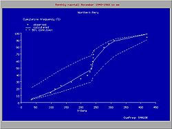
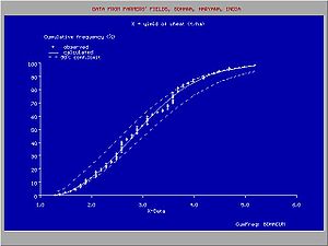
The figure gives an example of a useful introduction of a such a discontinuous distribution for rainfall data in northern Peru, where the climate is subject to the behavior Pacific ocean current El Niño. When the Niño extends to the south of Ecuador and enters the ocean along the coast of Peru, the climate in Northern Peru becomes tropical and wet. When the Niño does not reach Peru, the climate is semi−arid. For this reason, the higher rainfalls follow a different frequency distribution than the lower rainfalls.
The answer is yes, provided that the environmental conditions do not change. If the environmental conditions do change, such as alterations in the infrastructure of the river's watershed or in the rainfall pattern due to climatic changes, the prediction on the basis of the historical record is subject to a systematic error.
Even when there is no systematic error, there may be a random error
, because by chance the observed discharges during 1950 − 2000 may have been higher or lower than normal, while on the other hand the discharges from 2000 to 2050 may by chance be lower or higher than normal.
can help to estimate the range in which the random error may be.
In the case of cumulative frequency there are only two possibilities: a certain reference value X is exceeded or it is not exceeded. The sum of exceedance frequency and cumulative frequency is 1 or 100%. Therefore the binomial distribution can be used in estimating the range of the random error.
According to the normal theory, the binomial distribution can be approximated and for large N standard deviation Sd can be calculated as follows:
where Pc is the cumulative probability and N is the number of data. It is seen that the standard deviation Sd reduces at an increasing number of observations N.
The determination of the confidence interval
of Pc makes use of Student's t-test
(t). The value of t depends on the number of data and the confidence level of the estimate of the confidence interval. Then, the lower (L) and upper (U) confidence limits of Pc in a symmetrical distribution are found from:
This is known as Wald interval .
However, the binomial distribution is only symmetrical around the mean when Pc = 0.5, but it becomes asymmetrical
and more and more skew when Pc approaches 0 or 1. Therefore, by approximation, Pc and 1−Pc can be used as weight factors in the assignation of t.Sd to L and U :
where it can be seen that these expressions for Pc = 0.5 are the same as the previous ones.
Wald interval is known to perform poorly .
Wilson score interval provides confidence interval for binomial distributions based on score tests and has better sample coverage, see and binomial proportion confidence interval
for a more detailed overview.
 The cumulative probability Pc can also be called probability of non−exceedance. The probability of exceedance Pe is found from:
The return period
T defined as:
and indicates the expected number of observations that have to be done again to find the value of the variable in study greater than the value used for T.
The upper (TU) and lower (TL) confidence limits of return period
s can be found respectively as:
For extreme values of the variable in study, U is close to 1 and small changes in U originate large changes in TU. Hence, the estimated return period of extreme values is subject to a large random error. Moreover, the confidence intervals found hold for a long term prediction. For predictions at a shorter run, the confidence intervals U−L and TU−TL may actually be wider. Together with the limited certainty (less than 100%) used in the t−test, this explains why, for example, a 100−year rainfall might occur twice in 10 years.
The strict notion of return period actually has a meaning only when it concerns a time−dependent phenomenon, like point rainfall. The return period then corresponds to the expected waiting time until the exceedance occurs again. The return period has the same dimension as the length of time for which each observation is representative. For example, when the observations concern daily rainfalls, the return period is expressed in days, and for yearly rainfalls it is in years.
The confidence belt around an experimental cumulative frequency or return period curve gives an impression of the region in which the true distribution may be found.
Also, it clarifies that the experimentally found best fitting probability distribution may deviate from the true distribution.
 The observed data can be arranged in classes or groups with serial number k. Each group has a lower limit (Lk) and an upper limit (Uk). When the class (k) contains mk data and the total number of data is N, then the relative class or group frequency is found from:
or briefly:
or in percentage:
The presentation of all class frequencies gives a frequency distribution
or histogram
. Histograms, even when made from the same record, are different for different class limits.
The histogram can also be derived from the fitted cumulative probability distribution:
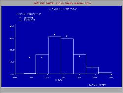
There may be a difference between Fgk and Pgk due to the deviations of the observed data from the fitted distribution (see figure).
Estimation theory
Estimation theory is a branch of statistics and signal processing that deals with estimating the values of parameters based on measured/empirical data that has a random component. The parameters describe an underlying physical setting in such a way that their value affects the distribution of the...
to exceedance probability (or equivalently to its complement). The complement, the non-exceedance probability concerns the frequency of occurrence of values of a phenomenon staying below a reference value. The phenomenon may be time or space dependent. Cumulative frequency is also called frequency of non−exceedance.
Cumulative frequency analysis
Frequency analysis
In cryptanalysis, frequency analysis is the study of the frequency of letters or groups of letters in a ciphertext. The method is used as an aid to breaking classical ciphers....
is done to obtain insight into how often a certain phenomenon (feature) is below a certain value. This may help in describing or explaining a situation in which the phenomenon is involved, or in planning interventions, for example in flood protection.
Definition
Frequency analysis applies to a record of observed data on a variable phenomenon. The record may be time dependent (e.g. rainfall measured in one spot) or space dependent (e.g. crop yields in an area) or otherwise.The variable phenomenon is modelled by a random variable
Random variable
In probability and statistics, a random variable or stochastic variable is, roughly speaking, a variable whose value results from a measurement on some type of random process. Formally, it is a function from a probability space, typically to the real numbers, which is measurable functionmeasurable...
and the parameterParameter
Parameter from Ancient Greek παρά also “para” meaning “beside, subsidiary” and μέτρον also “metron” meaning “measure”, can be interpreted in mathematics, logic, linguistics, environmental science and other disciplines....
of interest is the non-exceeding probability:in which
is a given reference value.The record of observed data consists of a random sample
Random sample
In statistics, a sample is a subject chosen from a population for investigation; a random sample is one chosen by a method involving an unpredictable component...
taken from .In this context the number of times the reference value
is not exceeded in the sample is called the cumulative frequency MXr. The relative cumulative frequency is this number divided by the sample size and is sometimes denoted as Fc(X≤Xr), or briefly as Fc(Xr). It is calculatd as;Briefly the expression can be noted as:
When Xr=Xmax, where Xmax is the maximum value observed, it is found that Fc=1, because M=N.
Estimation
The parameter is estimatedEstimator
In statistics, an estimator is a rule for calculating an estimate of a given quantity based on observed data: thus the rule and its result are distinguished....
on the basis of the relative cumulative frequency Fc. The estimate is:
In brief:
- Fc = M / (N+1)
The denominator N+1 is introduced instead of N to create the possibility for X to be greater than Xmax as now Pc(Xmax) is less than 1.
There exist also other proposals for the denominator (see plotting positions), but they are claimed to be incorrect.
Continuous distributions
To present the cumulative frequency distribution as a continuous mathematical equation instead of a discrete set of data, one may try to fit the cumulative frequency distribution to a known cumulative probability distribution,.If successful, the known equation is enough to report the frequency distribution and a table of data will not be required. Further, the equation helps interpolation and extrapolation.However, care should be taken with extrapolating a cumulative frequency distribution, because this may be a source of errors. One possible error is that the frequency distribution does not follow the selected probability distribution any more beyond the range of the observed data.
Any equation that gives the value 1 when integrated from a lower limit to an upper limit agreeing well with the data range, can be used as a probability distribution for fitting. A sample of probability distributions that may be used can be found in probability distributions.
Probability distributions can be fitted by several methods, for example:
- the parametric method, determining the parameters like mean and standard deviation from the X data using the method of moments, the maximum likelihood method and the method of probability weighted momentsL-momentIn statistics, L-moments are statistics used to summarize the shape of a probability distribution. They are analogous to conventional moments in that they can be used to calculate quantities analogous to standard deviation, skewness and kurtosis, termed the L-scale, L-skewness and L-kurtosis...
. - the regression method, linearizing the probability distribution through transformation and determining the parameters from a linear regression of the transformed Pc (obtained from ranking) on the transformed X data.
Application of both types of methods using for example the
- the normal distribution, the lognormal distribution, the logistic distribution, the loglogistic distribution, the exponential distributionExponential distributionIn probability theory and statistics, the exponential distribution is a family of continuous probability distributions. It describes the time between events in a Poisson process, i.e...
, the Fréchet distribution, the Gumbel distribution, the Pareto distribution, the Weibull distribution and other
often shows that a number of distributions fit the data well and do not yield significantly different results, while the differences between them may be small compared to the width of the confidence interval. This illustrates that it may be difficult to determine which distribution gives better results.
Discontinuous distributions
Sometimes it is possible to fit one type of probability distribution to the lower part of the data range and another type to the higher part, separated by a breakpoint, whereby the overall fit is improved.The figure gives an example of a useful introduction of a such a discontinuous distribution for rainfall data in northern Peru, where the climate is subject to the behavior Pacific ocean current El Niño. When the Niño extends to the south of Ecuador and enters the ocean along the coast of Peru, the climate in Northern Peru becomes tropical and wet. When the Niño does not reach Peru, the climate is semi−arid. For this reason, the higher rainfalls follow a different frequency distribution than the lower rainfalls.
Uncertainty
When a cumulative frequency distribution is derived from a record of data, it can be questioned if it can be used for predictions. For example, given a distribution of river discharges for the years 1950 to 2000, can this distribution be used to predict how often a certain river discharge will be exceeded in the years 2000 to 2050?The answer is yes, provided that the environmental conditions do not change. If the environmental conditions do change, such as alterations in the infrastructure of the river's watershed or in the rainfall pattern due to climatic changes, the prediction on the basis of the historical record is subject to a systematic error.
Even when there is no systematic error, there may be a random error
Random error
Random errors are errors in measurement that lead to measurable values being inconsistent when repeated measures of a constant attribute or quantity are taken...
, because by chance the observed discharges during 1950 − 2000 may have been higher or lower than normal, while on the other hand the discharges from 2000 to 2050 may by chance be lower or higher than normal.
Confidence intervals
Probability theoryProbability theory
Probability theory is the branch of mathematics concerned with analysis of random phenomena. The central objects of probability theory are random variables, stochastic processes, and events: mathematical abstractions of non-deterministic events or measured quantities that may either be single...
can help to estimate the range in which the random error may be.
In the case of cumulative frequency there are only two possibilities: a certain reference value X is exceeded or it is not exceeded. The sum of exceedance frequency and cumulative frequency is 1 or 100%. Therefore the binomial distribution can be used in estimating the range of the random error.
According to the normal theory, the binomial distribution can be approximated and for large N standard deviation Sd can be calculated as follows:
- Sd =√{Pc(1−Pc)/N}
where Pc is the cumulative probability and N is the number of data. It is seen that the standard deviation Sd reduces at an increasing number of observations N.
The determination of the confidence interval
Confidence interval
In statistics, a confidence interval is a particular kind of interval estimate of a population parameter and is used to indicate the reliability of an estimate. It is an observed interval , in principle different from sample to sample, that frequently includes the parameter of interest, if the...
of Pc makes use of Student's t-test
Student's t-test
A t-test is any statistical hypothesis test in which the test statistic follows a Student's t distribution if the null hypothesis is supported. It is most commonly applied when the test statistic would follow a normal distribution if the value of a scaling term in the test statistic were known...
(t). The value of t depends on the number of data and the confidence level of the estimate of the confidence interval. Then, the lower (L) and upper (U) confidence limits of Pc in a symmetrical distribution are found from:
- L = Pc − t.Sd.
- U = Pc + t.Sd
This is known as Wald interval .
However, the binomial distribution is only symmetrical around the mean when Pc = 0.5, but it becomes asymmetrical
Asymmetry
Asymmetry is the absence of, or a violation of, symmetry.-In organisms:Due to how cells divide in organisms, asymmetry in organisms is fairly usual in at least one dimension, with biological symmetry also being common in at least one dimension....
and more and more skew when Pc approaches 0 or 1. Therefore, by approximation, Pc and 1−Pc can be used as weight factors in the assignation of t.Sd to L and U :
- L = Pc − 2Pc.t.Sd
- U = Pc + 2(1−Pc).t.Sd
where it can be seen that these expressions for Pc = 0.5 are the same as the previous ones.
| Example N = 25, Pc = 0.8, Sd = 0.08, confidence level is 90%, t = 1.71, L = 0.70, U = 0.85 Thus, with 90% confidence, it is found that 0.70 < Pc < 0.85 Still, there is 10% chance that Pc < 0.70, or Pc > 0.85 |
Wald interval is known to perform poorly .
Wilson score interval provides confidence interval for binomial distributions based on score tests and has better sample coverage, see and binomial proportion confidence interval
Binomial proportion confidence interval
In statistics, a binomial proportion confidence interval is a confidence interval for a proportion in a statistical population. It uses the proportion estimated in a statistical sample and allows for sampling error. There are several formulas for a binomial confidence interval, but all of them rely...
for a more detailed overview.
Return period
- Pe = 1 − Pc.
The return period
Return period
A return period also known as a recurrence interval is an estimate of the interval of time between events like an earthquake, flood or river discharge flow of a certain intensity or size. It is a statistical measurement denoting the average recurrence interval over an extended period of time, and...
T defined as:
- T = 1/Pe
and indicates the expected number of observations that have to be done again to find the value of the variable in study greater than the value used for T.
The upper (TU) and lower (TL) confidence limits of return period
Return period
A return period also known as a recurrence interval is an estimate of the interval of time between events like an earthquake, flood or river discharge flow of a certain intensity or size. It is a statistical measurement denoting the average recurrence interval over an extended period of time, and...
s can be found respectively as:
- TU = 1/(1−U)
- TL = 1/(1−L)
For extreme values of the variable in study, U is close to 1 and small changes in U originate large changes in TU. Hence, the estimated return period of extreme values is subject to a large random error. Moreover, the confidence intervals found hold for a long term prediction. For predictions at a shorter run, the confidence intervals U−L and TU−TL may actually be wider. Together with the limited certainty (less than 100%) used in the t−test, this explains why, for example, a 100−year rainfall might occur twice in 10 years.
The strict notion of return period actually has a meaning only when it concerns a time−dependent phenomenon, like point rainfall. The return period then corresponds to the expected waiting time until the exceedance occurs again. The return period has the same dimension as the length of time for which each observation is representative. For example, when the observations concern daily rainfalls, the return period is expressed in days, and for yearly rainfalls it is in years.
Need of confidence belts
The figure shows the variation that may occur when obtaining samples of a variate that follows a certain probability distribution. The data were provided by Benson .The confidence belt around an experimental cumulative frequency or return period curve gives an impression of the region in which the true distribution may be found.
Also, it clarifies that the experimentally found best fitting probability distribution may deviate from the true distribution.
Histogram
- Fg(Lk<X≤Uk) = mk / N
or briefly:
- Fgk = m/N
or in percentage:
- Fg(%) = 100m/N
The presentation of all class frequencies gives a frequency distribution
Frequency distribution
In statistics, a frequency distribution is an arrangement of the values that one or more variables take in a sample. Each entry in the table contains the frequency or count of the occurrences of values within a particular group or interval, and in this way, the table summarizes the distribution of...
or histogram
Histogram
In statistics, a histogram is a graphical representation showing a visual impression of the distribution of data. It is an estimate of the probability distribution of a continuous variable and was first introduced by Karl Pearson...
. Histograms, even when made from the same record, are different for different class limits.
The histogram can also be derived from the fitted cumulative probability distribution:
- Pgk = Pc(Uk) − Pc(Lk)
There may be a difference between Fgk and Pgk due to the deviations of the observed data from the fitted distribution (see figure).