Cost curve

In economics

Economics

Economics is the social science that analyzes the production, distribution, and consumption of goods and services. The term economics comes from the Ancient Greek from + , hence "rules of the house"...

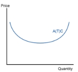
, a cost curve is a graph of the costs of production as a function of total quantity produced. In a free market

Free market

A free market is a competitive market where prices are determined by supply and demand. However, the term is also commonly used for markets in which economic intervention and regulation by the state is limited to tax collection, and enforcement of private ownership and contracts...

 economy, productively efficient

Productive efficiency

Productive efficiency occurs when the economy is utilizing all of its resources efficiently, producing most output from least input. The concept is illustrated on a production possibility frontier where all points on the curve are points of maximum productive efficiency...

 firms use these curves to find the optimal point of production (minimising cost), and profit maximizing

Profit maximization

In economics, profit maximization is the process by which a firm determines the price and output level that returns the greatest profit. There are several approaches to this problem...

 firms can use them to decide output quantities to achieve those aims. There are various types of cost curves, all related to each other, including total and average cost curves, and marginal ("for each additional unit") cost curves, which are the equal to the differential

Differentiation

Differentiation may refer to:* Differentiation , the process of finding a derivative* Differentiated instruction in education* Cellular differentiation in biology* Planetary differentiation in planetary science...

 of the total cost curves. Some are applicable to the short run, others to the long run.

Short-run average variable cost curve (SRAVC)

Average variable cost (which is a short-run concept) is the variable cost (typically labor cost) per unit of output: SRAVC = wL / Q where w is the wage rate, L is the quantity of labor used, and Q is the quantity of output produced. The SRAVC curve plots the short-run average variable cost against the level of output, and is typically drawn as U-shaped.

Short-run average total cost curve (SRATC or SRAC)

The average total cost curve is constructed to capture the relation between cost per unit of output and the level of output

Output

Output is the term denoting either an exit or changes which exit a system and which activate/modify a process. It is an abstract concept, used in the modeling, system design and system exploitation.-In control theory:...

, ceteris paribus

Ceteris paribus

or is a Latin phrase, literally translated as "with other things the same," or "all other things being equal or held constant." It is an example of an ablative absolute and is commonly rendered in English as "all other things being equal." A prediction, or a statement about causal or logical...

. A perfectly competitive and productively efficient firm organizes its factors of production

Factors of production

In economics, factors of production means inputs and finished goods means output. Input determines the quantity of output i.e. output depends upon input. Input is the starting point and output is the end point of production process and such input-output relationship is called a production function...

 in such a way that the average cost

Average cost

In economics, average cost or unit cost is equal to total cost divided by the number of goods produced . It is also equal to the sum of average variable costs plus average fixed costs...

 of production is at the lowest point. In the short run, when at least one factor of production is fixed, this occurs at the output level where it has enjoyed all possible average cost gains from increasing production. This is at the minimum point in the diagram on the right.

Short-run total cost is given by

STC = P_KK+P_LL,

where P_K is the unit price of using physical capital per unit time, P_L is the unit price of labor per unit time (the wage rate), K is the quantity of physical capital used, and L is the quantity of labor used. From this we obtain short-run average cost, denoted either SATC or SAC, as STC / Q:

SRATC or SRAC = P_KK/Q + P_LL/Q = P_K / AP_K + P_L / AP_L,

where AP_K = Q/K is the average product of capital and AP_L = Q/L is the average product of labor.

Short run average cost equals average fixed costs plus average variable costs. Average fixed cost continuously falls as production increases in the short run, because K is fixed in the short run. The shape of the average variable cost curve is directly determined by increasing and then diminishing marginal returns to the variable input (conventionally labor).

Long-run average cost curve (LRAC)

The long-run average cost curve depicts the cost per unit of output in the long run—that is, when all productive inputs' usage levels can be varied. All points on the line represent least-cost factor combinations; points above the line are attainable but unwise, while points below are unattainable given present factors of production. The behavioral assumption underlying the curve is that the producer will select the combination of inputs that will produce a given output at the lowest possible cost. Given that LRAC is an average quantity, one must not confuse it with the long-run marginal cost curve, which is the cost of one more unit. The LRAC curve is created as an envelope of an infinite number of short-run average total cost curves, each based on a particular fixed level of capital usage. The typical LRAC curve is U-shaped, reflecting increasing returns of scale where negatively-sloped, constant returns to scale where horizontal and decreasing returns (due to increases in factor prices) where positively sloped. Contrary to Viner, the envelope is not created by the minimum point of each short-run average cost curve. This mistake is recognized as Viner's Error.

In a long-run perfectly competitive

Perfect competition

In economic theory, perfect competition describes markets such that no participants are large enough to have the market power to set the price of a homogeneous product. Because the conditions for perfect competition are strict, there are few if any perfectly competitive markets...

 environment, the equilibrium level of output corresponds to the minimum efficient scale

Minimum Efficient Scale

Minimum efficient scale or efficient scale of production is a term used in industrial organization to denote the smallest output that a plant can produce such that its long run average costs are minimized.-Computing:...

, marked as Q2 in the diagram. This is due to the zero-profit requirement of a perfectly competitive equilibrium. This result, which implies production is at a level corresponding to the lowest possible average cost, does not imply that production levels other than that at the minimum point are not efficient. All points along the LRAC are productively efficient, by definition, but not all are equilibrium points in a long-run perfectly competitive environment.

In some industries, the bottom of the LRAC curve is large in comparison to market size (that is to say, for all intents and purposes, it is always declining and economies of scale exist indefinitely). This means that the largest firm tends to have a cost advantage, and the industry tends naturally to become a monopoly, and hence is called a natural monopoly

Natural monopoly

A monopoly describes a situation where all sales in a market are undertaken by a single firm. A natural monopoly by contrast is a condition on the cost-technology of an industry whereby it is most efficient for production to be concentrated in a single form...

. Natural monopolies tend to exist in industries with high capital costs in relation to variable costs, such as water supply

Water supply

Water supply is the provision of water by public utilities, commercial organisations, community endeavours or by individuals, usually via a system of pumps and pipes...

 and electricity supply.

Short-run marginal cost curve (SRMC)

A short-run marginal cost

Marginal cost

In economics and finance, marginal cost is the change in total cost that arises when the quantity produced changes by one unit. That is, it is the cost of producing one more unit of a good...

 curve graphically represents the relation between marginal (i.e., incremental) cost incurred by a firm in the short-run production of a good or service and the quantity of output produced. This curve is constructed to capture the relation between marginal cost and the level of output, holding other variables, like technology and resource prices, constant. The marginal cost curve is U-shaped. Marginal cost is relatively high at small quantities of output; then as production increases, marginal cost declines, reaches a minimum value, then rises. The marginal cost is shown in relation to marginal revenue, the incremental amount of sales revenue that an additional unit of the product or service will bring to the firm. This shape of the marginal cost curve is directly attributable to increasing, then decreasing marginal returns (and the law of diminishing marginal returns

Diminishing returns

In economics, diminishing returns is the decrease in the marginal output of a production process as the amount of a single factor of production is increased, while the amounts of all other factors of production stay constant.The law of diminishing returns In economics, diminishing returns (also...

). Marginal cost equals w/MP_L. For most production processes the marginal product of labor initially rises, reaches a maximum value and then continuously falls as production increases. Thus marginal cost initially falls, reaches a minimum value and then increases. The marginal cost curve intersects both the average variable cost curve and (short-run) average total cost curve at their minimum points. When the marginal cost curve is above an average cost curve the average curve is rising. When the marginal costs curve is below an average curve the average curve is falling. This relation holds regardless of whether the marginal curve is rising or falling.

Long-run marginal cost curve (LRMC)

The long-run marginal cost curve shows for each unit of output the added total cost incurred in the long run, that is, the conceptual period when all factors of production are variable so as minimize long-run average total cost. Stated otherwise, LRMC is the minimum increase in total cost associated with an increase of one unit of output when all inputs are variable.

The long-run marginal cost curve is shaped by economies and diseconomies of scale, a long-run concept, rather than the law of diminishing marginal returns, which is a short-run concept. The long-run marginal cost curve tends to be flatter than its short-run counterpart due to increased input flexibility as to cost minimization. The long-run marginal cost curve intersects the long-run average cost curve at the minimum point of the latter. When long-run marginal costs are below long-run average costs, long-run average costs are falling (as to additional units of output). When long-run marginal costs are above long run average costs, average costs are rising. Long-run marginal cost equals short run marginal-cost at the least-long-run-average-cost level of production. LRMC is the slope of the LR total-cost function.

Graphing cost curves together

Cost curves can be combined to provide information about firms. In this diagram for example, firms are assumed to be in a perfectly competitive

Perfect competition

In economic theory, perfect competition describes markets such that no participants are large enough to have the market power to set the price of a homogeneous product. Because the conditions for perfect competition are strict, there are few if any perfectly competitive markets...

 market. In a perfectly competitive market the price that firms are faced with would be the price at which the marginal cost curve cuts the average cost curve.

Cost curves and production functions

Assuming that factor prices are constant, the production function determines all cost functions. The variable cost curve is the inverted short-run production function or total product curve and its behavior and properties are determined by the production function. The slope of the short-run production function equals the marginal product of the variable input, conventionally labor. The slope of the variable cost function is marginal costs. The relationship between MC and the marginal product of labor MP_L is MC = w/MP_L. Because the wage rate w is assumed to be constant the shape of the variable cost curve is completely dependent on the marginal product of labor. The short-run total cost curve is simply the variable cost curve plus fixed costs. Because the production function determines the variable cost function it necessarily determines the shape and properties of marginal cost curve and the average cost curves.

If the firm is a perfect competitor in all input markets, and thus the per-unit prices of all its inputs are unaffected by how much of the inputs the firm purchases, then it can be shown that at a particular level of output, the firm has economies of scale (i.e., is operating in a downward sloping region of the long-run average cost curve) if and only if it has increasing returns to scale

Returns to scale

In economics, returns to scale and economies of scale are related terms that describe what happens as the scale of production increases in the long run, when all input levels including physical capital usage are variable...

. Likewise, it has diseconomies of scale (is operating in an upward sloping region of the long-run average cost curve) if and only if it has decreasing returns to scale, and has neither economies nor diseconomies of scale if it has constant returns to scale. In this case, with perfect competition in the output market the long-run market equilibrium will involve all firms operating at the minimum point of their long-run average cost curves (i.e., at the borderline between economies and diseconomies of scale).

If, however, the firm is not a perfect competitor in the input markets, then the above conclusions are modified. For example, if there are increasing returns to scale in some range of output levels, but the firm is so big in one or more input markets that increasing its purchases of an input drives up the input's per-unit cost, then the firm could have diseconomies of scale in that range of output levels. Conversely, if the firm is able to get bulk discounts of an input, then it could have economies of scale in some range of output levels even if it has decreasing returns in production in that output range.

Relationship between different curves

• Total Cost = Fixed Costs (FC) + Variable Costs (VC)
• Marginal Cost (MC) = dC/dQ; MC equals the slope of the total cost function and of the variable cost function
• Average Total Cost (ATC) = Total Cost/Q
• Average Fixed Cost (AFC) = FC/Q
• Average Variable Cost = VC/Q.
• ATC = AFC + AVC
• The MC curve is related to the shape of the ATC and AVC curves:
  • At a level of Q at which the MC curve is above the average total cost or average variable cost curve, the latter curve is rising.
  • If MC is below average total cost or average variable cost, then the latter curve is falling.
  • If MC equals average total cost, then average total cost is at its minimum value.
  • If MC equals average variable cost, then average variable cost is at its minimum value.

Relationship between short run and long run cost curves

Basic: For each quantity of output there is one cost minimizing level of capital and a unique short run average cost curve associated with producing the given quantity.

• Each STC curve can be tangent to the LRTC curve at only one point. The STC curve cannot cross (intersect) the LRTC curve. The STC curve can lie wholly “above” the LRTC curve with no tangency point.
• One STC curve is tangent to LRTC at the long-run cost minimizing level of production. At the point of tangency LRTC = STC. At all other levels of production STC will exceed LRTC.
• Average cost functions are the total cost function divided by the level of output. Therefore the SATC curveis also tangent to the LRATC curve at the cost-minimizing level of output. At the point of tangency LRATC = SATC. At all other levels of production SATC > LRATC To the left of the point of tangency the firm is using too much capital and fixed costs are too high. To the right of the point of tangency the firm is using too little capital and diminishing returns to labor are causing costs to increase.
• The slope of the total cost curves equals marginal cost. Therefore when STC is tangent to LTC, SMC = LRMC.
• At the long run cost minimizing level of output LRTC = STC; LRATC = SATC and LRMC = SMC, .
• The long run cost minimizing level of output may be different from minimum SATC, .
• With fixed unit costs of inputs, if the production function has constant returns to scale, then at the minimal level of the SATC curve we have SATC = LRATC = SMC = LRMC.
• With fixed unit costs of inputs, if the production function has increasing returns to scale, the minimum of the SATC curve is to the right of the point of tangency between the LRAC and the SATC curves. Where LRTC = STC, LRATC = SATC and LRMC = SMC.
• With fixed unit costs of inputs and decreasing returns the minimum of the SATC curve is to the left of the point of tangency between LRAC and SATC. Where LRTC = STC, LRATC = SATC and LRMC = SMC.
• With fixed unit input costs, a firm that is experiencing increasing (decreasing) returns to scale and is producing at its minimum SAC can always reduce average cost in the long run by expanding (reducing) the use of the fixed input.
• LRATC will always equal to or be less than SATC.
• If production process is exhibiting constant returns to scale then minimum SRAC equals minimum long run average cost. The LRAC and SRAC intersect at their common minimum values. Thus under constant returns to scale SRMC = LRMC = LRAC = SRAC .
• If the production process is experiencing decreasing or increasing, minimum short run average cost does not equal minimum long run average cost. If increasing returns to scale exist long run minimum will occur at a lower level of output than SRAC. This is because there are economies of scale that have not been exploited so in the long run a firm could always produce a quantity at a price lower than minimum short run aveage cost simply by using a larger plant.
• With decreasing returns, minimum SRAC occurs at a lower production level than minimum LRAC because a firm could reduce average costs by simply decreasing the size or its operations.
• The minimum of a SRAC occurs when the slope is zero. Thus the points of tangency between the U-shaped LRAC curve and the minimum of the SRAC curve would coincide only with that portion of the LRAC curve exhibiting constant economies of scale. For increasing returns to scale the point of tangency between the LRAC and the SRAc would have to occur at a level of output below level associated with the minimum of the SRAC curve.

These statements assume that the firm is using the optimal level of capital for the quantity produced. If not, then the SRAC curve would lie "wholly above" the LRAC and would not be tangent at any point.

U-shaped curves

Both the SRAC and LRAC curves are typically expressed as U-shaped. However, the shapes of the curves are not due to the same factors. For the short run curve the initial downward slope is largely due to declining average fixed costs. Increasing returns to the variable input at low levels of production also play a role, while the upward slope is due to diminishing marginal returns to the variable input. With the long run curve the shape by definition reflects economies and diseconomies of scale. At low levels of production long run production functions generally exhibit increasing returns to scale, which, for firms that are perfect competitors in input markets, means that the long run average cost is falling; the upward slope of the long run average cost function at higher levels of output is due to decreasing returns to scale at those output levels.

See also

• Cost
  Cost
  In production, research, retail, and accounting, a cost is the value of money that has been used up to produce something, and hence is not available for use anymore. In business, the cost may be one of acquisition, in which case the amount of money expended to acquire it is counted as cost. In this...
  
  
• Economic cost
  Economic cost
  The economic cost of a decision depends on both the cost of the alternative chosen and the benefit that the best alternative would have provided if chosen. Economic cost differs from accounting cost because it includes opportunity cost....
  
  
• Point of total assumption
  Point of total assumption
  The point of total assumption is a point on the cost line of the Profit-cost curve determined by the contract elements associated with a fixed price plus incentive-Firm Target contract above which the seller effectively bears all the costs of a cost overrun...
  
  
• Joel Dean (economist)
  Joel Dean (economist)
  Joel Dean is best known for his contributions to Corporate Finance theory in general, and particularly to the area of Capital budgeting. He is regarded as one of the founders of business economics...