Conjugate gradient method - AbsoluteAstronomy.com

Mathematics

Mathematics is the study of quantity, space, structure, and change. Mathematicians seek out patterns and formulate new conjectures. Mathematicians resolve the truth or falsity of conjectures by mathematical proofs, which are arguments sufficient to convince other mathematicians of their validity...

, the conjugate gradient method is an algorithm

Algorithm

In mathematics and computer science, an algorithm is an effective method expressed as a finite list of well-defined instructions for calculating a function. Algorithms are used for calculation, data processing, and automated reasoning...

for the numerical solution of particular systems of linear equations, namely those whose matrix is symmetric and positive-definite

Positive-definite matrix

In linear algebra, a positive-definite matrix is a matrix that in many ways is analogous to a positive real number. The notion is closely related to a positive-definite symmetric bilinear form ....

. The conjugate gradient method is an iterative method

Iterative method

In computational mathematics, an iterative method is a mathematical procedure that generates a sequence of improving approximate solutions for a class of problems. A specific implementation of an iterative method, including the termination criteria, is an algorithm of the iterative method...

, so it can be applied to sparse

Sparse matrix

In the subfield of numerical analysis, a sparse matrix is a matrix populated primarily with zeros . The term itself was coined by Harry M. Markowitz....

systems that are too large to be handled by direct methods such as the Cholesky decomposition

Cholesky decomposition

In linear algebra, the Cholesky decomposition or Cholesky triangle is a decomposition of a Hermitian, positive-definite matrix into the product of a lower triangular matrix and its conjugate transpose. It was discovered by André-Louis Cholesky for real matrices...

. Such systems often arise when numerically solving partial differential equation

Partial differential equation

In mathematics, partial differential equations are a type of differential equation, i.e., a relation involving an unknown function of several independent variables and their partial derivatives with respect to those variables...

s.

The conjugate gradient method can also be used to solve unconstrained optimization problems such as energy minimization

Energy minimization

In computational chemistry, energy minimization methods are used to compute the equilibrium configuration of molecules and solids....

. It was developed by Hestenes and Stiefel.

The biconjugate gradient method

Biconjugate gradient method

In mathematics, more specifically in numerical linear algebra, the biconjugate gradient method is an algorithm to solve systems of linear equationsA x= b.\,...

provides a generalization to non-symmetric matrices. Various nonlinear conjugate gradient method

Nonlinear conjugate gradient method

In numerical optimization, the nonlinear conjugate gradient method generalizes the conjugate gradient method to nonlinear optimization. For a quadratic function \displaystyle f:The minimum of f is obtained when the gradient is 0:...

s seek minima of nonlinear equations.

Description of the method

Suppose we want to solve the following system of linear equations

Ax = b

where the n-by-n matrix A is symmetric (i.e., A^T = A), positive definite (i.e., x^TAx > 0 for all non-zero vectors x in Rⁿ), and real

Real number

In mathematics, a real number is a value that represents a quantity along a continuum, such as -5 , 4/3 , 8.6 , √2 and π...

.

We denote the unique solution of this system by x_*.

The conjugate gradient method as a direct method

We say that two non-zero vectors u and v are conjugate

Inner automorphism

In abstract algebra an inner automorphism is a functionwhich, informally, involves a certain operation being applied, then another one performed, and then the initial operation being reversed...

(with respect to A) if

Since A is symmetric and positive definite, the left-hand side defines an inner product

Inner product space

In mathematics, an inner product space is a vector space with an additional structure called an inner product. This additional structure associates each pair of vectors in the space with a scalar quantity known as the inner product of the vectors...

So, two vectors are conjugate if they are orthogonal with respect to this inner product.
Being conjugate is a symmetric relation: if u is conjugate to v, then v is conjugate to u.
(Note: This notion of conjugate is not related to the notion of complex conjugate

Complex conjugate

In mathematics, complex conjugates are a pair of complex numbers, both having the same real part, but with imaginary parts of equal magnitude and opposite signs...

.)

Suppose that {p_k} is a sequence of n mutually conjugate directions. Then the p_k form a basis

Basis (linear algebra)

In linear algebra, a basis is a set of linearly independent vectors that, in a linear combination, can represent every vector in a given vector space or free module, or, more simply put, which define a "coordinate system"...

of Rⁿ, so we can expand the solution x_* of Ax = b in this basis:

The coefficients are given by

(because

are mutually conjugate)

This result is perhaps most transparent by considering the inner product defined above.

This gives the following method for solving the equation Ax = b: find a sequence of n conjugate directions, and then compute the coefficients α_k.

The conjugate gradient method as an iterative method

If we choose the conjugate vectors p_k carefully, then we may not need all of them to obtain a good approximation to the solution x_*. So, we want to regard the conjugate gradient method as an iterative method. This also allows us to solve systems where n is so large that the direct method would take too much time.

We denote the initial guess for x_* by x₀. We can assume without loss of generality that x₀ = 0 (otherwise, consider the system Az = b − Ax₀ instead). Starting with x₀ we search for the solution and in each iteration we need a metric to tell us whether we are closer to the solution x_* (that is unknown to us). This metric comes from the fact that the solution x_* is also the unique minimizer of the following quadratic function

Quadratic function

A quadratic function, in mathematics, is a polynomial function of the formf=ax^2+bx+c,\quad a \ne 0.The graph of a quadratic function is a parabola whose axis of symmetry is parallel to the y-axis....

; so if f(x) becomes smaller in an iteration it means that we are closer to x_*.

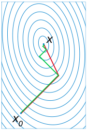
This suggests taking the first basis vector p₁ to be the negative of the gradient of f at x = x₀. This gradient equals Ax₀−b. Since x₀ = 0, this means we take p₁ = b. The other vectors in the basis will be conjugate to the gradient, hence the name conjugate gradient method.

Let r_k be the residual at the kth step:

Note that r_k is the negative gradient of f at x = x_k, so the gradient descent

Gradient descent

Gradient descent is a first-order optimization algorithm. To find a local minimum of a function using gradient descent, one takes steps proportional to the negative of the gradient of the function at the current point...

method would be to move in the direction r_k. Here, we insist that the directions p_k be conjugate to each other. We also require the next search direction is built out of the current residue and all previous search directions, which is reasonable enough in practice.

The conjugation constraint is an orthonormal-type constraint and hence the algorithm bears resemblance to Gram-Schmidt orthonormalization

Gram–Schmidt process

In mathematics, particularly linear algebra and numerical analysis, the Gram–Schmidt process is a method for orthonormalising a set of vectors in an inner product space, most commonly the Euclidean space Rn...

.

This gives the following expression:

(see the picture at the top of the article for the effect of the conjugacy constraint on convergence). Following this direction, the next optimal location is given by

with

where the last equality holds because p_k+1 and x_k are conjugate.

The resulting algorithm

The above algorithm gives the most straightforward explanation towards the conjugate gradient method. However, it requires storage of all the previous searching directions and residue vectors, and many matrix vector multiplications, thus could be computationally expensive. In practice, one modifies slightly the condition obtaining the last residue vector, not to minimize the metric following the search direction, but instead to make it orthogonal to the previous residue. Minimization of the metric along the search direction will be obtained automatically in this case.
One can then result in an algorithm which only requires storage of the last two residue vectors and the last search direction, and only one matrix vector multiplication. Note that the algorithm described below is equivalent to the
previously discussed straightforward procedure.

The algorithm is detailed below for solving Ax = b where A is a real, symmetric, positive-definite matrix. The input vector x₀ can be an approximate initial solution or 0.

repeat

if r_k+1 is sufficiently small then exit loop end if

end repeat

The result is x_k+1

This is the most commonly used algorithm. The same formula for

is also used in the Fletcher–Reeves nonlinear conjugate gradient method

Nonlinear conjugate gradient method

Example code in GNU Octave

function [x] = conjgrad(A,b,x)
r=b-A*x;
p=r;
rsold=r'*r;

for i=1:size(A)(1)
Ap=A*p;
alpha=rsold/(p'*Ap);
x=x+alpha*p;
r=r-alpha*Ap;
rsnew=r'*r;
if sqrt(rsnew)<1e-10
break;
end
p=r+rsnew/rsold*p;
rsold=rsnew;
end
end

Numerical example

To illustrate the conjugate gradient method, we will complete a simple example.

Considering the linear system Ax = b given by

we will perform two steps of the conjugate gradient method beginning with the initial guess

in order to find an approximate solution to the system.

Solution

Our first step is to calculate the residual vector r₀ associated with x₀. This residual is computed from the formula r₀ = b - Ax₀, and in our case is equal to

Since this is the first iteration, we will use the residual vector r₀ as our initial search direction p₀; the method of selecting p_k will change in further iterations.

We now compute the scalar α₀ using the relationship

We can now compute x₁ using the formula

This result completes the first iteration, the result being an "improved" approximate solution to the system, x₁. We may now move on and compute the next residual vector r₁ using the formula

Our next step in the process is to compute the scalar β₀ that will eventually be used to determine the next search direction p₁.

Now, using this scalar β₀, we can compute the next search direction p₁ using the relationship

We now compute the scalar α₁ using our newly-acquired p₁ using the same method as that used for α₀.

Finally, we find x₂ using the same method as that used to find x₁.

The result, x₂, is a "better" approximation to the system's solution than x₁ and x₀. If exact arithmetic were to be used in this example instead of limited-precision, then the exact solution would theoretically have been reached after n = 2 iterations (n being the order of the system).

Convergence properties of the conjugate gradient method

The conjugate gradient method can theoretically be viewed as a direct method, as it produces the exact solution after a finite number of iterations, which is not larger than the size of the matrix, in the absence of round-off error

Round-off error

A round-off error, also called rounding error, is the difference between the calculated approximation of a number and its exact mathematical value. Numerical analysis specifically tries to estimate this error when using approximation equations and/or algorithms, especially when using finitely many...

. However, the conjugate gradient method is unstable with respect to even small perturbations, e.g., most directions are not in practice conjugate, and the exact solution is never obtained. Fortunately, the conjugate gradient method can be used as an iterative method

Iterative method

as it provides monotonically improving approximations

to the exact solution, which may reach the required tolerance after a relatively small (compared to the problem size) number of iterations. The improvement is typically linear and its speed is determined by the condition number

Condition number

In the field of numerical analysis, the condition number of a function with respect to an argument measures the asymptotically worst case of how much the function can change in proportion to small changes in the argument...

of the system matrix

: the larger is

, the slower the improvement .

If

is large, preconditioning is used to replace the original system

with

so that

gets smaller than

, see below.

The preconditioned conjugate gradient method

In most cases, preconditioning is necessary to ensure fast convergence of the conjugate gradient method. The preconditioned conjugate gradient method takes the following form:

repeat

if r_k+1 is sufficiently small then exit loop end if

end repeat

The result is x_k+1

The above formulation is equivalent to applying the conjugate gradient method without preconditioning to the system

where

and

.

The preconditioner matrix M has to be symmetric positive-definite and fixed, i.e., cannot change from iteration to iteration.
If any of these assumptions on the preconditioner is violated, the behavior of the preconditioned conjugate gradient method may become unpredictable.

The flexible preconditioned conjugate gradient method

In numerically challenging applications, sophisticated preconditioners are used, which may lead to variable preconditioning, changing between iterations. Even if the preconditioner is symmetric positive-definite on every iteration, the fact that it may change makes the arguments above invalid, and in practical tests leads to a significant slow down of the convergence of the algorithm presented above. Using the Polak–Ribière

Nonlinear conjugate gradient method

formula

instead of the Fletcher–Reeves

Nonlinear conjugate gradient method

formula

may dramatically improve the convergence in this case. This version of the preconditioned conjugate gradient method can be called flexible, as it allows for variable preconditioning. The implementation of the flexible version requires storing an extra vector. For a fixed preconditioner,

so both formulas for

are equivalent in exact arithmetic, i.e., without the round-off error

Round-off error

.

The mathematical explanation of the better convergence behavior of the method with the Polak–Ribière

Nonlinear conjugate gradient method

formula is that the method is locally optimal in this case, in particular, it converges not slower than the locally optimal steepest descent method.

The conjugate gradient method vs. the locally optimal steepest descent method

In both the original and the preconditioned conjugate gradient methods one only needs to always set

in order to turn them into locally optimal, using the line search, steepest descent methods. With this substitution, vectors

are always the same as vectors

, so there is no need to store vectors

. Thus, every iteration of these steepest descent methods is a bit cheaper compared to that for the conjugate gradient methods. However, the latter converge faster, unless a (highly) variable preconditioner

Preconditioner

In mathematics, preconditioning is a procedure of an application of a transformation, called the preconditioner, that conditions a given problem into a form that is more suitable for numerical solution. Preconditioning is typically related to reducing a condition number of the problem...

is used, see above.

Derivation of the method

The conjugate gradient method can be derived from several different perspectives, including specialization of the conjugate direction method for optimization, and variation of the Arnoldi

Arnoldi iteration

In numerical linear algebra, the Arnoldi iteration is an eigenvalue algorithm and an important example of iterative methods. Arnoldi finds the eigenvalues of general matrices; an analogous method for Hermitian matrices is the Lanczos iteration. The Arnoldi iteration was invented by W. E...

/Lanczos iteration for eigenvalue problems. Despite differences in their approaches, these derivations share a common topic—proving the orthogonality of the residuals and conjugacy of the search directions. These two properties are crucial to developing the well-known succinct formulation of the method.

Conjugate gradient on the normal equations

The conjugate gradient method can be applied to an arbitrary n-by-m matrix by applying it to normal equations A^TA and right-hand side vector A^Tb, since A^TA is a symmetric positive-semidefinite matrix for any A. The result is conjugate gradient on the normal equations (CGNR).

A^TAx = A^Tb

As an iterative method, it is not necessary to form A^TA explicitly in memory but only to perform the matrix-vector and transpose matrix-vector multiplications. Therefore CGNR is particularly useful when A is a sparse matrix

Sparse matrix

In the subfield of numerical analysis, a sparse matrix is a matrix populated primarily with zeros . The term itself was coined by Harry M. Markowitz....

since these operations are usually extremely efficient. However the downside of forming the normal equations is that the condition number

Condition number

κ(A^TA) is equal to κ²(A) and so the rate of convergence of CGNR may be slow and the quality of the approximate solution may be sensitive to roundoff errors. Finding a good preconditioner

Preconditioner

is often an important part of using the CGNR method.

Several algorithms have been proposed (e.g., CGLS, LSQR). The LSQR algorithm purportedly has the best numerical stability when A is ill-conditioned, i.e., A has a large condition number

Condition number

External links

An Introduction to the Conjugate Gradient Method Without the Agonizing Pain by Jonathan Richard Shewchuk.
Iterative methods for sparse linear systems by Yousef Saad
LSQR: Sparse Equations and Least Squares by Christopher Paige and Michael Saunders.

The source of this article is wikipedia, the free encyclopedia. The text of this article is licensed under the GFDL.

Description of the method

The conjugate gradient method as a direct method

The conjugate gradient method as an iterative method

The resulting algorithm

Example code in GNU Octave

Numerical example

Solution

Convergence properties of the conjugate gradient method

The preconditioned conjugate gradient method

The flexible preconditioned conjugate gradient method

The conjugate gradient method vs. the locally optimal steepest descent method

Derivation of the method

Conjugate gradient on the normal equations

See also

External links