

Cayley–Hamilton theorem
Encyclopedia
In linear algebra
, the Cayley–Hamilton theorem (named after the mathematicians Arthur Cayley
and William Hamilton
) states that every square matrix over a commutative ring
(such as the real
or complex
field
) satisfies its own characteristic equation
.
More precisely:
If A is a given n×n matrix and In is the n×n identity matrix
, then the characteristic polynomial
of A is defined as

where "det" is the determinant
operation. Since the entries of the matrix are (linear or constant) polynomials in λ, the determinant is also a polynomial in λ. The Cayley–Hamilton theorem states that "substituting" the matrix A for λ in this polynomial results in the zero matrix:

The powers of λ that have become powers of A by the substitution should be computed by repeated matrix multiplication, and the constant term should be multiplied by the identity matrix (the zeroth power of A) so that it can be added to the other terms.
The theorem allows An to be expressed as a linear combination of the lower matrix powers of A.
When the ring is a field, the Cayley–Hamilton theorem is equivalent to the statement that the minimal polynomial
of a square matrix divides its characteristic polynomial.
 .
.
Its characteristic polynomial is given by
The Cayley–Hamilton theorem claims that, if we define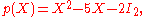
then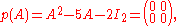
which one can verify easily.
For a 2×2 matrix,
the characteristic polynomial is given by p(λ)=λ2−(a+d)λ+(ad−bc), so the Cayley–Hamilton theorem states that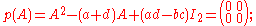
which is indeed always the case, evident by working out the entries of A2.
For a general n×n invertible matrix A, i.e., one with nonzero determinant, A−1 can thus be written as an (n−1)-th order polynomial expression
in A: As indicated, the Cayley–Hamilton theorem amounts to the identity
with cn−1=−tr(A), etc., where tr(A) is the trace
of the matrix A.
This can then be written as
and, by multiplying both sides by , one is led to the compact expression for the inverse
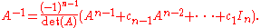
For larger matrices, the expressions for the coefficients ck of the characteristic polynomial in terms of the matrix components become increasingly complicated; but they can also be expressed in terms of traces of powers of the matrix A, using Newton's identities
(at least when the ring contains the rational numbers), thus resulting in more compact expressions (but which involve divisions by certain integers).
For instance, in the above 2×2 matrix example, the coefficient −c1=a+d of λ above is just the trace of A, trA, while the constant coefficient c0=ad−bc can be written as ½((trA)2−tr(A2)). (Of course, it is also the determinant of A in this case.)
In fact, this expression, ½((trA)2−tr(A2)), always gives the coefficient cn−2 of λn−2 in the characteristic polynomial of any n×n matrix; so, for a 3×3 matrix A, the statement of the Cayley–Hamilton theorem can also be written as
where the right-hand side designates a 3×3 matrix with all entries reduced to zero.
Similarly, one can write for a 4×4 matrix A:
and so on for larger matrices, with the increasingly complex expressions for the coefficients deducible from Newton's identities.
An alternate, practical method for obtaining these coefficients ck for a general n×n matrix, yielding the above ones virtually by inspection, relies on .
.
Hence,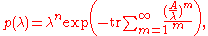
where the exponential only needs be expanded to order λ−n, since p(λ) is of order n. (Again, this requires a ring containing the rational numbers.)
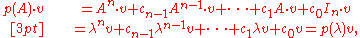
The Cayley–Hamilton theorem always provides a relationship between the powers of A (though not always the simplest one), which allows one to simplify expressions involving such powers, and evaluate them without having to compute the power An or any higher powers of A.
For instance the concrete 2×2 Example above can be written as
Then, for example, to calculate A4, observe

 requires two steps: first the coefficients ci of the characteristic polynomial are determined by development as a polynomial in t of the determinant
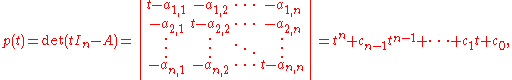
and then these coeffcients are used in a linear combination of powers of A that is equated to the n×n null matrix: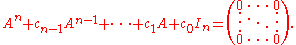
The left hand side can be worked out to an n×n matrix whose entries are (enormous) polynomial expressions in the set of entries of A, so the Cayley–Hamilton theorem states that each of these
  expressions are equivalent to 0. For any fixed value of n these identities can be obtained by tedious but completely straightforward algebraic manipulations. None of these computations can show however why the Cayley–Hamilton theorem should be valid for matrices of all possible sizes n, so a uniform proof for all n is needed.
 , then
which is the null vector since (the eigenvalues of A are precisely the roots of p(t)). This holds for all possible eigenvalues λ, so the two matrices equated by the theorem certainly give the same (null) result when applied to any eigenvector. Now if A admits a basis
of eigenvectors, in other words if A is diagonalizable, then the Cayley–Hamilton theorem must hold for A, since two matrices that give the same values when applied to each element of a basis must be equal. Not all matrices are diagonalizable, but for matrices with complex coefficients many of them are: the set of diagonalizable complex square matrices of a given size is dense
in the set of all such square matrices (for a matrix to be diagonalizable it suffices for instance that its characteristic polynomial not have multiple roots). Now if any of the expressions that the theorem equates to 0 would not reduce to a null expression, in other words if it would be a nonzero polynomial in the coefficients of the matrix, then the set of complex matrices for which this expression happens to give 0 would not be dense in the set of all matrices, which would contradict the fact that the theorem holds for all diagonalizable matrices. Thus one can see that the Cayley–Hamilton theorem must be true.
While this provides a valid proof (for matrices over the complex numbers), the argument is not very satisfactory, since the identities represented by the theorem do not in any way depend on the nature of the matrix (diagonalizable or not), nor on the kind of entries allowed (for matrices with real entries the diagonizable ones do not form a dense set, and it seems strange one would have to consider complex matrices to see that the Cayley–Hamilton theorem holds for them). We shall therefore now consider only arguments that prove the theorem directly for any matrix using algebraic manipulations only; these also have the benefit of working for matrices with entries in any commutative ring
.
There is a great variety of such proofs of the Cayley–Hamilton theorem, of which several will be given here. They vary in the amount of abstract algebraic notions required to understand the proof. The simplest proofs use just those notions needed to formulate the theorem (matrices, polynomials with numeric entries, determinants), but involve technical computations that render somewhat mysterious the fact that they lead precisely to the correct conclusion. It is possible to avoid such details, but at the price of involving more subtle algebraic notions: polynomials with coefficients in a non-commutative ring, or matrices with unusual kinds of entries.
 of an n×n matrix M. This is a matrix whose coefficients are given by polynomial expressions in the coefficients of M (in fact by certain (n − 1)×(n − 1) determinants), in such a way that one has the following fundamental relations
These relations are a direct consequence of the basic properties of determinants: evaluation of the (i,j) entry of the matrix product on the left gives the expansion by column j of the determinant of the matrix obtained from M by replacing column i by a copy of column j, which is if
if  and zero otherwise; the matrix product on the right is similar, but for expansions by rows. Being a consequence of just algebraic expression manipulation, these relations are valid for matrices with entries in any commutative ring (commutativity must be assumed for determinants to be defined in the first place). This is important to note here, because these relations will be applied for matrices with non-numeric entries such as polynomials.
 whose determinant is the characteristic polynomial of A is such a matrix, and since polynomials form a commutative ring, it has an adjugate
Then according to the right hand fundamental relation of the adjugate one has
Since B is also a matrix with polynomials in t as entries, one can for each i collect the coefficients of in each entry to form a matrix Bi of numbers, such that one has
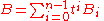
(the way the entries of B are defined makes clear that no powers higher than occur). While this looks like a polynomial with matrices as coefficients, we shall not consider such a notion; it is just a way to write a matrix with polynomial entries as linear combination of constant matrices, and the coefficient
  has been written to the left of the matrix to stress this point of view. Now one can expand the matrix product in our equation by bilinearity
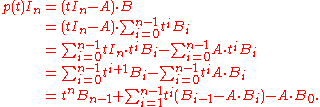
Writing , one obtains an equality of two matrices with polynomial entries, written as linear combinations of constant matrices with powers of t as coefficients. Such an equality can hold only if in any matrix position the entry that is multiplied by a given power
  is the same on both sides; it follows that the constant matrices with coefficient
  in both expressions must be equal. Writing these equations for i from n down to 0 one finds
We multiply the equation of the coefficients of ti from the left by Ai, and sum up; the left-hand sides form a telescoping sum and cancel completely, which results in the equation
This completes the proof.
Let M = Mn(R) be the ring of n × n matrices with entries in some ring R (such as the real or complex numbers) that has A as an element. Matrices with as coefficients polynomials in t, such as or its adjugate B in the first proof, are elements of Mn(R[t]). By collecting like powers of t, such matrices can be written as "polynomials" in t with constant matrices as coefficients; write M[t] for the set of such polynomials. Since this set is in bijection with Mn(R[t]), one defines arithmetic operations on it correspondingly, in particular multiplication is given by
respecting the order of the coefficient matrices from the two operands; obviously this gives a non-commutative multiplication. Thus the identity
from the first proof can be viewed as one involving a multiplication of elements in M[t].
At this point, it is tempting to set t equal to the matrix A, which makes the first factor on the left equal to the null matrix, and the right hand side equal to p(A); however, this is not an allowed operation when coefficients do not commute. It is possible to define a "right-evaluation map" evA : M[t] → M, which replaces each ti by the matrix power Ai of A, where one stipulates that the power is always to be multiplied on the right to the corresponding coefficient. However this map is not a ring homomorphism: the right-evaluation of a product differs in general from the product of the right-evaluations. This is so because multiplication of polynomials with matrix coefficients does not model multiplication of expressions containing unknowns: a product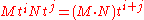 is defined assuming that t commutes with N, but this may fail if t is replaced by the matrix A.
One can work around this difficulty in the particular situation at hand, since the above right-evaluation map does become a ring homomorphism if the matrix A is in the center
of the ring of coefficients, so that it commutes with all the coefficients of the polynomials (the argument proving this is straightforward, exactly because commuting t with coefficients is now justified after evaluation). Now A is not always in the center of M, but we may replace M with a smaller ring provided it contains all the coefficients of the polynomials in question: , A, and the coefficients
  of the polynomial B. The obvious choice for such a subring is the centralizer Z of A, the subring of all matrices that commute with A; by definition A is in the center of Z. This centralizer obviously contains
  , and A, but one has to show that it contains the matrices
  . To do this one combines the two fundamental relations for adjugates, writing out the adjugate B as a polynomial:
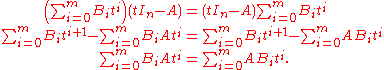
Equating the coefficients shows that for each i, we have A Bi = Bi A as desired. Having found the proper setting in which evA is indeed a homomorphism of rings, one can complete the proof as suggested above: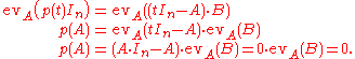
This completes the proof.
 on the left by the monic polynomial
  , while the final equation expresses the fact that the remainder is zero. This division is performed in the ring of polynomials with matrix coefficients. Indeed, even over a non-commutative ring, Euclidean division by a monic polynomial P is defined, and always produces a unique quotient and remainder with the same degree condition as in the commutative case, provided it is specified at which side one wishes P to be a factor (here that is to the left). To see that quotient and remainder are unique (which is the important part of the statement here), it suffices to write
 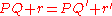 as
as 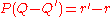 and observe that since P is monic,
  cannot have a degree less than that of P, unless
  .
.
But the dividend and divisor
  used here both lie in the subring (R[A])[t], where R[A] is the subring of the matrix ring M generated by A: the R-linear span of all powers of A. Therefore the Euclidean division can in fact be performed within that commutative polynomial ring, and of course it then gives the same quotient B and remainder 0 as in the larger ring; in particular this shows that B in fact lies in
  . But in this commutative setting it is valid to set t to A in the equation
  , in other words apply the evaluation map
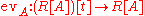
which is a ring homomorphism, giving
just like in the second proof, as desired.
In addition to proving the theorem, the above argument tells us that the coefficients of B are polynomials in A, while from the second proof we only knew that they lie in the centralizer Z of A; in general Z is a larger subring than R[A], and not necessarily commutative. In particular the constant term
  lies in R[A]. Since A is an arbitrary square matrix, this proves that
  can always be expressed as a polynomial in
  (with coefficients that depend on
  ), something that is not obvious from the definition of the adjugate matrix. In fact the equations found in the first proof allow successively expressing
  , ...,
  ,
,  as polynomials in A, which leads to the identity
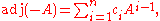
valid for all n×n matrices, where is the characteristic polynomial of A. Note that this identity implies the statement of the Cayley–Hamilton theorem: one may move
  to the right hand side, multiply the resulting equation (on the left or on the right) by
  , and use the fact that
 in statement of the theorem is obtained by first evaluating the determinant and then substituting the matrix A for t; doing that subtitution into the matrix
  before evaluating the determinant is not meaningful. Nevertheless, it is possible to give an interpretation where
  is obtained directly as the value of a certain deteminant, but this requires a more complicated setting, one of matrices over a ring in which one can interpret both the entries
  of A, and all of A itself. One could take for this the ring M of n × n matrices over R, where the entry
  is realised as
  , and A as itself. But considering matrices with matrices as entries might cause confusion with block matrices
, which is not intended, as that gives the wrong notion of determinant (recall that the determinant of a matrix is defined as a sum of products of its entries, and in the case of a block matrix this is generally not the same as the corresponding sum of products of its blocks!). It is clearer to distinguish A from the endomorphism φ of an n-dimensional vector space V (or free R-module if R is not a field) defined by it in a basis e1, ..., en, and to take matrices over the ring End(V) of all such endomorphisms. Then is a possible matrix entry, while A designates the element of
  whose
whose  entry is endomorphism of scalar multiplication by
  ; similarly In will be interpreted as element of
  . However, since End(V) is not a commutative ring, no deteminant is defined on
  ; this can only be done for matrices over a commutative subring of End(V). Now the entries of the matrix
  all lie in the subring R[φ] generated by the identity and φ, which is commutative. Then a determinant map
  is defined, and
  evaluates to the value p(φ) of the characteristic polynomial of A at φ (this holds independently of the relation between A and φ); the Cayley–Hamilton theorem states that p(φ) is the null endomorphism.
In this form, the following proof can be obtained from that of (which in fact is the more general statement related to the Nakayama lemma
; one takes for the ideal in that proposition the whole ring R). The fact that A is the matrix of φ in the basis e1, ..., en means that
One can interpret these as n components of one equation in Vn, whose members can be written using the matrix-vector product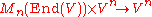 that is defined as usual, but with individual entries
  and
and  being "multiplied" by forming
  ; this gives:
where is the element whose component i is ei (in other words it is the basis e1, ..., en of V written as a column of vectors). Writing this equation as
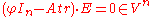
one recognizes the transpose
of the matrix considered above, and its determinant (as element of
  ) is also p(φ). To derive from this equation that
  , one left-multiplies by the adjugate matrix
of , which is defined in the matrix ring
  , giving
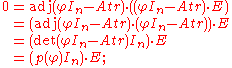
the associativity of matrix-matrix and matrix-vector multiplication used in the first step is a purely formal property of those operations, independent of the nature of the entries. Now component i of this equation says that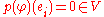 ; thus p(φ) vanishes on all ei, and since these elements generate V it follows that
  , completing the proof.
One additional fact that follows from this proof is that the matrix A whose characteristic polynomial is taken need not be identical to the value φ substituted into that polynomial; it suffices that φ be an endomorphism of V satisfying the initial equations φ(ei) = Σj Aj,iej for some sequence of elements e1,...,en that generate V (which space might have smaller dimension than n, or in case the ring R is not a field it might not be a free module
at all).
and substitute for
for  , obtaining

There are many ways to see why this argument is wrong. First, in Cayley–Hamilton theorem, p(A) is an n×n matrix. However, the right hand side of the above equation is the value of a determinant, which is a scalar. So they cannot be equated unless n = 1 (i.e. A is just a scalar). Second, in the expression , the variable
  actually occurs at the diagonal entries of the matrix
  . To illustrate, consider the characteristic polynomial in the previous example again:
If one substitutes the entire matrix for
for  in those positions, one obtains
in which the "matrix" expression is simply not a valid one. Note, however, that if scalar multiples of identity matrices
instead of scalars are subtracted in the above, i.e. if the substitution is performed as
then the determinant is indeed zero, but the expanded matrix in question does not evaluate to ; nor can its determinant (a scalar) be compared to
  (a matrix). So the argument that
  still does not apply.
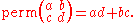
Actually, if such an argument holds, it should also hold when other multilinear forms instead of determinant is used. For instance, if we consider the permanent
function and define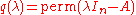 , then by the same argument, we should be able to "prove" that q(A) = 0. But this statement is demonstrably wrong. In the 2-dimensional case, for instance, the permanent of a matrix is given by
So, for the matrix in the previous example,

Yet one can verify that
One of the proofs for Cayley–Hamilton theorem above bears some similarity to the argument that . By introducing a matrix with non-numeric coefficients, one can actually let
  lives inside a matrix entry, but then
  is not equal to
  , and the conclusion is reached differently.
 for j = 1,...,n. This more general version of the theorem is the source of the celebrated Nakayama lemma
in commutative algebra and algebraic geometry.
Linear algebra
Linear algebra is a branch of mathematics that studies vector spaces, also called linear spaces, along with linear functions that input one vector and output another. Such functions are called linear maps and can be represented by matrices if a basis is given. Thus matrix theory is often...
, the Cayley–Hamilton theorem (named after the mathematicians Arthur Cayley
Arthur Cayley
Arthur Cayley F.R.S. was a British mathematician. He helped found the modern British school of pure mathematics....
and William Hamilton
William Rowan Hamilton
Sir William Rowan Hamilton was an Irish physicist, astronomer, and mathematician, who made important contributions to classical mechanics, optics, and algebra. His studies of mechanical and optical systems led him to discover new mathematical concepts and techniques...
) states that every square matrix over a commutative ring
Commutative ring
In ring theory, a branch of abstract algebra, a commutative ring is a ring in which the multiplication operation is commutative. The study of commutative rings is called commutative algebra....
(such as the real
Real number
In mathematics, a real number is a value that represents a quantity along a continuum, such as -5 , 4/3 , 8.6 , √2 and π...
or complex
Complex number
A complex number is a number consisting of a real part and an imaginary part. Complex numbers extend the idea of the one-dimensional number line to the two-dimensional complex plane by using the number line for the real part and adding a vertical axis to plot the imaginary part...
field
Field (mathematics)
In abstract algebra, a field is a commutative ring whose nonzero elements form a group under multiplication. As such it is an algebraic structure with notions of addition, subtraction, multiplication, and division, satisfying certain axioms...
) satisfies its own characteristic equation
Characteristic equation
Characteristic equation may refer to:* Characteristic equation , used to solve linear differential equations* Characteristic equation, a characteristic polynomial equation in linear algebra used to find eigenvalues...
.
More precisely:
If A is a given n×n matrix and In is the n×n identity matrix
Identity matrix
In linear algebra, the identity matrix or unit matrix of size n is the n×n square matrix with ones on the main diagonal and zeros elsewhere. It is denoted by In, or simply by I if the size is immaterial or can be trivially determined by the context...
, then the characteristic polynomial
Characteristic polynomial
In linear algebra, one associates a polynomial to every square matrix: its characteristic polynomial. This polynomial encodes several important properties of the matrix, most notably its eigenvalues, its determinant and its trace....
of A is defined as
where "det" is the determinant
Determinant
In linear algebra, the determinant is a value associated with a square matrix. It can be computed from the entries of the matrix by a specific arithmetic expression, while other ways to determine its value exist as well...
operation. Since the entries of the matrix are (linear or constant) polynomials in λ, the determinant is also a polynomial in λ. The Cayley–Hamilton theorem states that "substituting" the matrix A for λ in this polynomial results in the zero matrix:
The powers of λ that have become powers of A by the substitution should be computed by repeated matrix multiplication, and the constant term should be multiplied by the identity matrix (the zeroth power of A) so that it can be added to the other terms.
The theorem allows An to be expressed as a linear combination of the lower matrix powers of A.
When the ring is a field, the Cayley–Hamilton theorem is equivalent to the statement that the minimal polynomial
Minimal polynomial (linear algebra)
In linear algebra, the minimal polynomial of an n-by-n matrix A over a field F is the monic polynomial P over F of least degree such that P=0...
of a square matrix divides its characteristic polynomial.
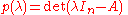
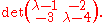
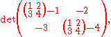
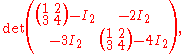
Example
As a concrete example, let.Its characteristic polynomial is given by
The Cayley–Hamilton theorem claims that, if we define
then
which one can verify easily.
Illustration for specific dimensions and practical applications
For a 1×1 matrix A = (a), the characteristic polynomial is given by p(λ)=λ−a, and so p(A)=(a)−a(1)=(0) is obvious.For a 2×2 matrix,
the characteristic polynomial is given by p(λ)=λ2−(a+d)λ+(ad−bc), so the Cayley–Hamilton theorem states that
which is indeed always the case, evident by working out the entries of A2.
For a general n×n invertible matrix A, i.e., one with nonzero determinant, A−1 can thus be written as an (n−1)-th order polynomial expression
Polynomial expression
In mathematics, and in particular in the field of algebra, a polynomial expression in one or more given entities E1, E2, ..., is any meaningful expression constructed from copies of those entities together with constants, using the operations of addition and multiplication...
in A: As indicated, the Cayley–Hamilton theorem amounts to the identity
with cn−1=−tr(A), etc., where tr(A) is the trace
Trace (linear algebra)
In linear algebra, the trace of an n-by-n square matrix A is defined to be the sum of the elements on the main diagonal of A, i.e.,...
of the matrix A.
This can then be written as
and, by multiplying both sides by
, one is led to the compact expression for the inverseFor larger matrices, the expressions for the coefficients ck of the characteristic polynomial in terms of the matrix components become increasingly complicated; but they can also be expressed in terms of traces of powers of the matrix A, using Newton's identities
Newton's identities
In mathematics, Newton's identities, also known as the Newton–Girard formulae, give relations between two types of symmetric polynomials, namely between power sums and elementary symmetric polynomials...
(at least when the ring contains the rational numbers), thus resulting in more compact expressions (but which involve divisions by certain integers).
For instance, in the above 2×2 matrix example, the coefficient −c1=a+d of λ above is just the trace of A, trA, while the constant coefficient c0=ad−bc can be written as ½((trA)2−tr(A2)). (Of course, it is also the determinant of A in this case.)
In fact, this expression, ½((trA)2−tr(A2)), always gives the coefficient cn−2 of λn−2 in the characteristic polynomial of any n×n matrix; so, for a 3×3 matrix A, the statement of the Cayley–Hamilton theorem can also be written as
where the right-hand side designates a 3×3 matrix with all entries reduced to zero.
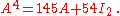
Similarly, one can write for a 4×4 matrix A:
and so on for larger matrices, with the increasingly complex expressions for the coefficients deducible from Newton's identities.
An alternate, practical method for obtaining these coefficients ck for a general n×n matrix, yielding the above ones virtually by inspection, relies on
.Hence,
where the exponential only needs be expanded to order λ−n, since p(λ) is of order n. (Again, this requires a ring containing the rational numbers.)
The Cayley–Hamilton theorem always provides a relationship between the powers of A (though not always the simplest one), which allows one to simplify expressions involving such powers, and evaluate them without having to compute the power An or any higher powers of A.
For instance the concrete 2×2 Example above can be written as
Then, for example, to calculate A4, observe
Proving the theorem in general
As the examples above show, obtaining the statement of the Cayley–Hamilton theorem for an n×n matrix requires two steps: first the coefficients ci of the characteristic polynomial are determined by development as a polynomial in t of the determinantand then these coeffcients are used in a linear combination of powers of A that is equated to the n×n null matrix:
The left hand side can be worked out to an n×n matrix whose entries are (enormous) polynomial expressions in the set of entries
of A, so the Cayley–Hamilton theorem states that each of these expressions are equivalent to 0. For any fixed value of n these identities can be obtained by tedious but completely straightforward algebraic manipulations. None of these computations can show however why the Cayley–Hamilton theorem should be valid for matrices of all possible sizes n, so a uniform proof for all n is needed.Preliminaries
If a vector v of size n happens to be an eigenvector of A with eigenvalue λ, in other words if, thenwhich is the null vector since
(the eigenvalues of A are precisely the roots of p(t)). This holds for all possible eigenvalues λ, so the two matrices equated by the theorem certainly give the same (null) result when applied to any eigenvector. Now if A admits a basisBasis (linear algebra)
In linear algebra, a basis is a set of linearly independent vectors that, in a linear combination, can represent every vector in a given vector space or free module, or, more simply put, which define a "coordinate system"...
of eigenvectors, in other words if A is diagonalizable, then the Cayley–Hamilton theorem must hold for A, since two matrices that give the same values when applied to each element of a basis must be equal. Not all matrices are diagonalizable, but for matrices with complex coefficients many of them are: the set of diagonalizable complex square matrices of a given size is dense
Dense set
In topology and related areas of mathematics, a subset A of a topological space X is called dense if any point x in X belongs to A or is a limit point of A...
in the set of all such square matrices (for a matrix to be diagonalizable it suffices for instance that its characteristic polynomial not have multiple roots). Now if any of the
expressions that the theorem equates to 0 would not reduce to a null expression, in other words if it would be a nonzero polynomial in the coefficients of the matrix, then the set of complex matrices for which this expression happens to give 0 would not be dense in the set of all matrices, which would contradict the fact that the theorem holds for all diagonalizable matrices. Thus one can see that the Cayley–Hamilton theorem must be true.While this provides a valid proof (for matrices over the complex numbers), the argument is not very satisfactory, since the identities represented by the theorem do not in any way depend on the nature of the matrix (diagonalizable or not), nor on the kind of entries allowed (for matrices with real entries the diagonizable ones do not form a dense set, and it seems strange one would have to consider complex matrices to see that the Cayley–Hamilton theorem holds for them). We shall therefore now consider only arguments that prove the theorem directly for any matrix using algebraic manipulations only; these also have the benefit of working for matrices with entries in any commutative ring
Commutative ring
In ring theory, a branch of abstract algebra, a commutative ring is a ring in which the multiplication operation is commutative. The study of commutative rings is called commutative algebra....
.
There is a great variety of such proofs of the Cayley–Hamilton theorem, of which several will be given here. They vary in the amount of abstract algebraic notions required to understand the proof. The simplest proofs use just those notions needed to formulate the theorem (matrices, polynomials with numeric entries, determinants), but involve technical computations that render somewhat mysterious the fact that they lead precisely to the correct conclusion. It is possible to avoid such details, but at the price of involving more subtle algebraic notions: polynomials with coefficients in a non-commutative ring, or matrices with unusual kinds of entries.
Adjugate matrices
All proofs below use the notion of the adjugate matrixAdjugate matrix
In linear algebra, the adjugate or classical adjoint of a square matrix is a matrix that plays a role similar to the inverse of a matrix; it can however be defined for any square matrix without the need to perform any divisions....
of an n×n matrix M. This is a matrix whose coefficients are given by polynomial expressions in the coefficients of M (in fact by certain (n − 1)×(n − 1) determinants), in such a way that one has the following fundamental relationsThese relations are a direct consequence of the basic properties of determinants: evaluation of the (i,j) entry of the matrix product on the left gives the expansion by column j of the determinant of the matrix obtained from M by replacing column i by a copy of column j, which is
if and zero otherwise; the matrix product on the right is similar, but for expansions by rows. Being a consequence of just algebraic expression manipulation, these relations are valid for matrices with entries in any commutative ring (commutativity must be assumed for determinants to be defined in the first place). This is important to note here, because these relations will be applied for matrices with non-numeric entries such as polynomials.A direct algebraic proof
This proof uses just the kind of objects needed to formulate the Cayley–Hamilton theorem: matrices with polynomials as entries. The matrix whose determinant is the characteristic polynomial of A is such a matrix, and since polynomials form a commutative ring, it has an adjugateThen according to the right hand fundamental relation of the adjugate one has
Since B is also a matrix with polynomials in t as entries, one can for each i collect the coefficients of
in each entry to form a matrix Bi of numbers, such that one has(the way the entries of B are defined makes clear that no powers higher than
occur). While this looks like a polynomial with matrices as coefficients, we shall not consider such a notion; it is just a way to write a matrix with polynomial entries as linear combination of constant matrices, and the coefficient has been written to the left of the matrix to stress this point of view. Now one can expand the matrix product in our equation by bilinearityWriting
, one obtains an equality of two matrices with polynomial entries, written as linear combinations of constant matrices with powers of t as coefficients. Such an equality can hold only if in any matrix position the entry that is multiplied by a given power is the same on both sides; it follows that the constant matrices with coefficient in both expressions must be equal. Writing these equations for i from n down to 0 one findsWe multiply the equation of the coefficients of ti from the left by Ai, and sum up; the left-hand sides form a telescoping sum and cancel completely, which results in the equation
This completes the proof.
A proof using polynomials with matrix coefficients
This proof is similar to the first one, but tries to give meaning to the notion of polynomial with matrix coefficients that was suggested by the expressions occurring in that proof. This requires considerable care, since it is somewhat unusual to consider polynomials with coefficients in a non-commutative ring, and not all reasoning that is valid for commutative polynomials can be applied in this setting. Notably, while arithmetic of polynomials over a commutative ring models the arithmetic of polynomial functions, this is not the case over a non-commutative ring (in fact there is no obvious notion of polynomial function in this case that is closed under multiplication). So when considering polynomials in t with matrix coefficients, the variable t must not be thought of as an "unknown", but as a formal symbol that is to be manipulated according to given rules; in particular one cannot just set t to a specific value.Let M = Mn(R) be the ring of n × n matrices with entries in some ring R (such as the real or complex numbers) that has A as an element. Matrices with as coefficients polynomials in t, such as
or its adjugate B in the first proof, are elements of Mn(R[t]). By collecting like powers of t, such matrices can be written as "polynomials" in t with constant matrices as coefficients; write M[t] for the set of such polynomials. Since this set is in bijection with Mn(R[t]), one defines arithmetic operations on it correspondingly, in particular multiplication is given byrespecting the order of the coefficient matrices from the two operands; obviously this gives a non-commutative multiplication. Thus the identity
from the first proof can be viewed as one involving a multiplication of elements in M[t].
At this point, it is tempting to set t equal to the matrix A, which makes the first factor on the left equal to the null matrix, and the right hand side equal to p(A); however, this is not an allowed operation when coefficients do not commute. It is possible to define a "right-evaluation map" evA : M[t] → M, which replaces each ti by the matrix power Ai of A, where one stipulates that the power is always to be multiplied on the right to the corresponding coefficient. However this map is not a ring homomorphism: the right-evaluation of a product differs in general from the product of the right-evaluations. This is so because multiplication of polynomials with matrix coefficients does not model multiplication of expressions containing unknowns: a product
is defined assuming that t commutes with N, but this may fail if t is replaced by the matrix A.One can work around this difficulty in the particular situation at hand, since the above right-evaluation map does become a ring homomorphism if the matrix A is in the center
Center (algebra)
The term center or centre is used in various contexts in abstract algebra to denote the set of all those elements that commute with all other elements. It is often denoted Z, from German Zentrum, meaning "center". More specifically:...
of the ring of coefficients, so that it commutes with all the coefficients of the polynomials (the argument proving this is straightforward, exactly because commuting t with coefficients is now justified after evaluation). Now A is not always in the center of M, but we may replace M with a smaller ring provided it contains all the coefficients of the polynomials in question:
, A, and the coefficients of the polynomial B. The obvious choice for such a subring is the centralizer Z of A, the subring of all matrices that commute with A; by definition A is in the center of Z. This centralizer obviously contains , and A, but one has to show that it contains the matrices . To do this one combines the two fundamental relations for adjugates, writing out the adjugate B as a polynomial:Equating the coefficients shows that for each i, we have A Bi = Bi A as desired. Having found the proper setting in which evA is indeed a homomorphism of rings, one can complete the proof as suggested above:
This completes the proof.
A synthesis of the first two proofs
In the first proof, one was able to determine the coefficients Bi of B based on the right hand fundamental relation for the adjugate only. In fact the first n equations derived can be interpreted as determining the quotient B of the Euclidean division of the polynomial on the left by the monic polynomial , while the final equation expresses the fact that the remainder is zero. This division is performed in the ring of polynomials with matrix coefficients. Indeed, even over a non-commutative ring, Euclidean division by a monic polynomial P is defined, and always produces a unique quotient and remainder with the same degree condition as in the commutative case, provided it is specified at which side one wishes P to be a factor (here that is to the left). To see that quotient and remainder are unique (which is the important part of the statement here), it suffices to write as and observe that since P is monic, cannot have a degree less than that of P, unless .But the dividend
and divisor used here both lie in the subring (R[A])[t], where R[A] is the subring of the matrix ring M generated by A: the R-linear span of all powers of A. Therefore the Euclidean division can in fact be performed within that commutative polynomial ring, and of course it then gives the same quotient B and remainder 0 as in the larger ring; in particular this shows that B in fact lies in . But in this commutative setting it is valid to set t to A in the equation , in other words apply the evaluation mapwhich is a ring homomorphism, giving
just like in the second proof, as desired.
In addition to proving the theorem, the above argument tells us that the coefficients
of B are polynomials in A, while from the second proof we only knew that they lie in the centralizer Z of A; in general Z is a larger subring than R[A], and not necessarily commutative. In particular the constant term lies in R[A]. Since A is an arbitrary square matrix, this proves that can always be expressed as a polynomial in (with coefficients that depend on ), something that is not obvious from the definition of the adjugate matrix. In fact the equations found in the first proof allow successively expressing , ..., , as polynomials in A, which leads to the identityvalid for all n×n matrices, where
is the characteristic polynomial of A. Note that this identity implies the statement of the Cayley–Hamilton theorem: one may move to the right hand side, multiply the resulting equation (on the left or on the right) by , and use the fact thatA proof using matrices of endomorphisms
As was mentioned above, the matrix in statement of the theorem is obtained by first evaluating the determinant and then substituting the matrix A for t; doing that subtitution into the matrix before evaluating the determinant is not meaningful. Nevertheless, it is possible to give an interpretation where is obtained directly as the value of a certain deteminant, but this requires a more complicated setting, one of matrices over a ring in which one can interpret both the entries of A, and all of A itself. One could take for this the ring M of n × n matrices over R, where the entry is realised as , and A as itself. But considering matrices with matrices as entries might cause confusion with block matricesBlock matrix
In the mathematical discipline of matrix theory, a block matrix or a partitioned matrix is a matrix broken into sections called blocks. Looking at it another way, the matrix is written in terms of smaller matrices. We group the rows and columns into adjacent 'bunches'. A partition is the rectangle...
, which is not intended, as that gives the wrong notion of determinant (recall that the determinant of a matrix is defined as a sum of products of its entries, and in the case of a block matrix this is generally not the same as the corresponding sum of products of its blocks!). It is clearer to distinguish A from the endomorphism φ of an n-dimensional vector space V (or free R-module if R is not a field) defined by it in a basis e1, ..., en, and to take matrices over the ring End(V) of all such endomorphisms. Then
is a possible matrix entry, while A designates the element of whose entry is endomorphism of scalar multiplication by ; similarly In will be interpreted as element of . However, since End(V) is not a commutative ring, no deteminant is defined on ; this can only be done for matrices over a commutative subring of End(V). Now the entries of the matrix all lie in the subring R[φ] generated by the identity and φ, which is commutative. Then a determinant map is defined, and evaluates to the value p(φ) of the characteristic polynomial of A at φ (this holds independently of the relation between A and φ); the Cayley–Hamilton theorem states that p(φ) is the null endomorphism.In this form, the following proof can be obtained from that of (which in fact is the more general statement related to the Nakayama lemma
Nakayama lemma
In mathematics, more specifically modern algebra and commutative algebra, Nakayama's lemma also known as the Krull–Azumaya theorem governs the interaction between the Jacobson radical of a ring and its finitely generated modules...
; one takes for the ideal in that proposition the whole ring R). The fact that A is the matrix of φ in the basis e1, ..., en means that
One can interpret these as n components of one equation in Vn, whose members can be written using the matrix-vector product
that is defined as usual, but with individual entries and being "multiplied" by forming ; this gives:where
is the element whose component i is ei (in other words it is the basis e1, ..., en of V written as a column of vectors). Writing this equation asone recognizes the transpose
Transpose
In linear algebra, the transpose of a matrix A is another matrix AT created by any one of the following equivalent actions:...
of the matrix
considered above, and its determinant (as element of ) is also p(φ). To derive from this equation that , one left-multiplies by the adjugate matrixAdjugate matrix
In linear algebra, the adjugate or classical adjoint of a square matrix is a matrix that plays a role similar to the inverse of a matrix; it can however be defined for any square matrix without the need to perform any divisions....
of
, which is defined in the matrix ring , givingthe associativity of matrix-matrix and matrix-vector multiplication used in the first step is a purely formal property of those operations, independent of the nature of the entries. Now component i of this equation says that
; thus p(φ) vanishes on all ei, and since these elements generate V it follows that , completing the proof.One additional fact that follows from this proof is that the matrix A whose characteristic polynomial is taken need not be identical to the value φ substituted into that polynomial; it suffices that φ be an endomorphism of V satisfying the initial equations φ(ei) = Σj Aj,iej for some sequence of elements e1,...,en that generate V (which space might have smaller dimension than n, or in case the ring R is not a field it might not be a free module
Free module
In mathematics, a free module is a free object in a category of modules. Given a set S, a free module on S is a free module with basis S.Every vector space is free, and the free vector space on a set is a special case of a free module on a set.-Definition:...
at all).
A bogus "proof": p(A) = det(AIn − A) = det(A − A) = 0
One elementary but incorrect argument for the theorem is to "simply" take the definitionand substitute
for , obtainingThere are many ways to see why this argument is wrong. First, in Cayley–Hamilton theorem, p(A) is an n×n matrix. However, the right hand side of the above equation is the value of a determinant, which is a scalar. So they cannot be equated unless n = 1 (i.e. A is just a scalar). Second, in the expression
, the variable actually occurs at the diagonal entries of the matrix . To illustrate, consider the characteristic polynomial in the previous example again:If one substitutes the entire matrix
for in those positions, one obtainsin which the "matrix" expression is simply not a valid one. Note, however, that if scalar multiples of identity matrices
instead of scalars are subtracted in the above, i.e. if the substitution is performed as
then the determinant is indeed zero, but the expanded matrix in question does not evaluate to
; nor can its determinant (a scalar) be compared to (a matrix). So the argument that still does not apply.Actually, if such an argument holds, it should also hold when other multilinear forms instead of determinant is used. For instance, if we consider the permanent
Permanent
The permanent of a square matrix in linear algebra, is a function of the matrix similar to the determinant. The permanent, as well as the determinant, is a polynomial in the entries of the matrix...
function and define
, then by the same argument, we should be able to "prove" that q(A) = 0. But this statement is demonstrably wrong. In the 2-dimensional case, for instance, the permanent of a matrix is given bySo, for the matrix
in the previous example,Yet one can verify that
One of the proofs for Cayley–Hamilton theorem above bears some similarity to the argument that
. By introducing a matrix with non-numeric coefficients, one can actually let lives inside a matrix entry, but then is not equal to , and the conclusion is reached differently.Abstraction and generalizations
The above proofs show that the Cayley–Hamilton theorem holds for matrices with entries in any commutative ring R, and that p(φ) = 0 will hold whenever φ is an endomorphism of an R module generated by elements e1,...,en that satisfies for j = 1,...,n. This more general version of the theorem is the source of the celebrated Nakayama lemmaNakayama lemma
In mathematics, more specifically modern algebra and commutative algebra, Nakayama's lemma also known as the Krull–Azumaya theorem governs the interaction between the Jacobson radical of a ring and its finitely generated modules...
in commutative algebra and algebraic geometry.
External links
- A proof from PlanetMath.
- The Cayley-Hamilton Theorem at MathPages