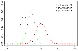
In
probability theoryProbability theory is the branch of mathematics concerned with analysis of random phenomena. The central objects of probability theory are random variables, stochastic processes, and events: mathematical abstractions of non-deterministic events or measured quantities that may either be single...
and
statisticsStatistics is the study of the collection, organization, analysis, and interpretation of data. It deals with all aspects of this, including the planning of data collection in terms of the design of surveys and experiments....
, the
binomial distribution is the discrete probability distribution of the number of successes in a sequence of
n independentIn probability theory, to say that two events are independent intuitively means that the occurrence of one event makes it neither more nor less probable that the other occurs...
yes/no experiments, each of which yields success with
probabilityProbability is ordinarily used to describe an attitude of mind towards some proposition of whose truth we arenot certain. The proposition of interest is usually of the form "Will a specific event occur?" The attitude of mind is of the form "How certain are we that the event will occur?" The...
p. Such a success/failure experiment is also called a Bernoulli experiment or
Bernoulli trialIn the theory of probability and statistics, a Bernoulli trial is an experiment whose outcome is random and can be either of two possible outcomes, "success" and "failure"....
; when
n = 1, the binomial distribution is a
Bernoulli distribution. The binomial distribution is the basis for the popular
binomial testIn statistics, the binomial test is an exact test of the statistical significance of deviations from a theoretically expected distribution of observations into two categories.-Common use:...
of
statistical significanceIn statistics, a result is called statistically significant if it is unlikely to have occurred by chance. The phrase test of significance was coined by Ronald Fisher....
.
The binomial distribution is frequently used to model the number of successes in a sample of size
n drawn with replacement from a population of size
N. If the sampling is carried out without replacement, the draws are not independent and so the resulting distribution is a
hypergeometric distribution, not a binomial one. However, for
N much larger than
n, the binomial distribution is a good approximation, and widely used.
Probability mass function
In general, if the random variable
K follows the binomial distribution with parameters
n and
p, we write
K ~ B(
n,
p). The probability of getting exactly
k successes in
n trials is given by the
probability mass functionIn probability theory and statistics, a probability mass function is a function that gives the probability that a discrete random variable is exactly equal to some value...
:
for
k = 0, 1, 2, ...,
n, where
is the
binomial coefficientIn mathematics, binomial coefficients are a family of positive integers that occur as coefficients in the binomial theorem. They are indexed by two nonnegative integers; the binomial coefficient indexed by n and k is usually written \tbinom nk , and it is the coefficient of the x k term in...
(hence the name of the distribution) "
n choose
k", also denoted
C(
n,
k),
nCk, or
nCk. The formula can be understood as follows: we want
k successes (
pk) and
n −
k failures (1 −
p)
n − k. However, the
k successes can occur anywhere among the
n trials, and there are C(
n,
k) different ways of distributing
k successes in a sequence of
n trials.
In creating reference tables for binomial distribution probability, usually the table is filled in up to
n/2 values. This is because for
k >
n/2, the probability can be calculated by its complement as
Looking at the expression
ƒ(
k,
n,
p) as a function of
k, there is a
k value that maximizes it. This
k value can be found by calculating

and comparing it to 1. There is always an integer
M that satisfies
ƒ(
k,
n,
p) is monotone increasing for
k <
M and monotone decreasing for
k >
M, with the exception of the case where (
n + 1)
p is an integer. In this case, there are two values for which
ƒ is maximal: (
n + 1)
p and (
n + 1)
p − 1.
M is the
most probable (
most likely) outcome of the Bernoulli trials and is called the
modeIn statistics, the mode is the value that occurs most frequently in a data set or a probability distribution. In some fields, notably education, sample data are often called scores, and the sample mode is known as the modal score....
. Note that the probability of it occurring can be fairly small.
Cumulative distribution function
The
cumulative distribution functionIn probability theory and statistics, the cumulative distribution function , or just distribution function, describes the probability that a real-valued random variable X with a given probability distribution will be found at a value less than or equal to x. Intuitively, it is the "area so far"...
can be expressed as:
where

is the "floor" under
x, i.e. the greatest integer less than or equal to
x.
It can also be represented in terms of the regularized incomplete beta function, as follows:
For
k ≤
np,
upper boundsIn probability theory, the Chernoff bound, named after Herman Chernoff, gives exponentially decreasing bounds on tail distributions of sums of independent random variables...
for the lower tail of the distribution function can be derived. In particular,
Hoeffding's inequalityIn probability theory, Hoeffding's inequality provides an upper bound on the probability for the sum of random variables to deviate from its expected value. Hoeffding's inequality was proved by Wassily Hoeffding.LetX_1, \dots, X_n \!...
yields the bound
and Chernoff's inequality can be used to derive the bound
Moreover, these bounds are reasonably tight when
p = 1/2, since the following expression holds for all
k ≥
3n/8
Mean and variance
If
X ~
B(
n,
p) (that is,
X is a binomially distributed random variable), then the
expected valueIn probability theory, the expected value of a random variable is the weighted average of all possible values that this random variable can take on...
of
X is
-

and the varianceIn probability theory and statistics, the variance is a measure of how far a set of numbers is spread out. It is one of several descriptors of a probability distribution, describing how far the numbers lie from the mean . In particular, the variance is one of the moments of a distribution...
is
-

This fact is easily proven as follows. Suppose first that we have a single Bernoulli trial. There are two possible outcomes: 1 and 0, the first occurring with probability p and the second having probability 1 − p. The expected value in this trial will be equal to . The variance in this trial is calculated similarly: .
The generic binomial distribution is a sum of n independent Bernoulli trials. The mean and the variance of such distributions are equal to the sums of means and variances of each individual trial:
-

Mode and median
Usually the modeIn statistics, the mode is the value that occurs most frequently in a data set or a probability distribution. In some fields, notably education, sample data are often called scores, and the sample mode is known as the modal score....
of a binomial B(n, p) distribution is equal to ⌊(n + 1)p⌋, where ⌊ ⌋ is the floor functionIn mathematics and computer science, the floor and ceiling functions map a real number to the largest previous or the smallest following integer, respectively...
. However when (n + 1)p is an integer and p is neither 0 nor 1, then the distribution has two modes: (n + 1)p and (n + 1)p − 1. When p is equal to 0 or 1, the mode will be 0 and n correspondingly. These cases can be summarized as follows:
-

In general, there is no single formula to find the medianIn probability theory and statistics, a median is described as the numerical value separating the higher half of a sample, a population, or a probability distribution, from the lower half. The median of a finite list of numbers can be found by arranging all the observations from lowest value to...
for a binomial distribution, and it may even be non-unique. However several special results have been established:
- If np is an integer, then the mean, median, and mode coincide and equal np.
- Any median m must lie within the interval ⌊np⌋ ≤ m ≤ ⌈np⌉.
- A median m cannot lie too far away from the mean: }.
- The median is unique and equal to m = round
Rounding a numerical value means replacing it by another value that is approximately equal but has a shorter, simpler, or more explicit representation; for example, replacing $23.4476 with $23.45, or the fraction 312/937 with 1/3, or the expression √2 with 1.414.Rounding is often done on purpose to...
(np) in cases when either or or |m − np| ≤ min{p, 1 − p} (except for the case when p = ½ and n is odd).
- When p = 1/2 and n is odd, any number m in the interval ½(n − 1) ≤ m ≤ ½(n + 1) is a median of the binomial distribution. If p = 1/2 and n is even, then m = n/2 is the unique median.
Covariance between two binomials
If two binomially distributed random variables X and Y are observed together, estimating their covariance can be useful. Using the definition of covarianceIn probability theory and statistics, covariance is a measure of how much two variables change together. Variance is a special case of the covariance when the two variables are identical.- Definition :...
, in the case n = 1 we have
-

The first term is non-zero only when both X and Y are one, and μX and μY are equal to the two probabilities. Defining pB as the probability of both happening at the same time, this gives
-

and for n such trials again due to independence
-

If X and Y are the same variable, this reduces to the variance formula given above.
Sums of binomials
If X ~ B(n, p) and Y ~ B(m, p) are independent binomial variables, then X + Y is again a binomial variable; its distribution is

Conditional binomials
If X ~ B(n, p) and, conditional on X, Y ~ B(X, q), then Y is a simple binomial variable with distribution

Bernoulli distribution
The Bernoulli distribution is a special case of the binomial distribution, where n = 1. Symbolically, X ~ B(1, p) has the same meaning as X ~ Bern(p). Conversely, any binomial distribution, B(n, p), is the sum of n independent Bernoulli trials, Bern(p), each with the same probability p.
Poisson binomial distribution
The binomial distribution is a special case of the Poisson binomial distribution, which is a sum of n independent non-identical Bernoulli trials Bern(pi). If X has the Poisson binomial distribution with p1 = … = pn =p then X ~ B(n, p).
Normal approximation
If n is large enough, then the skew of the distribution is not too great. In this case, if a suitable continuity correctionIn probability theory, if a random variable X has a binomial distribution with parameters n and p, i.e., X is distributed as the number of "successes" in n independent Bernoulli trials with probability p of success on each trial, then...
is used, then an excellent approximation to B(n, p) is given by the normal distribution

The approximation generally improves as n increases (at least 20) and is better when p is not near to 0 or 1. Various rules of thumbA rule of thumb is a principle with broad application that is not intended to be strictly accurate or reliable for every situation. It is an easily learned and easily applied procedure for approximately calculating or recalling some value, or for making some determination...
may be used to decide whether n is large enough, and p is far enough from the extremes of zero or one:
- One rule is that both x=np and n(1 − p) must be greater than 5. However, the specific number varies from source to source, and depends on how good an approximation one wants; some sources give 10 which gives virtually the same results as the following rule for large n until n is very large (ex: x=11, n=7752).
- That rule is that for the normal approximation is adequate if
-
-

- Another commonly used rule holds that the normal approximation is appropriate only if everything within 3 standard deviations of its mean is within the range of possible values, that is if
-
-

- Also as the approximation generally improves, it can be shown that the inflection point
In differential calculus, an inflection point, point of inflection, or inflection is a point on a curve at which the curvature or concavity changes sign. The curve changes from being concave upwards to concave downwards , or vice versa...
s occur at
-
-

The following is an example of applying a continuity correctionIn probability theory, if a random variable X has a binomial distribution with parameters n and p, i.e., X is distributed as the number of "successes" in n independent Bernoulli trials with probability p of success on each trial, then...
: Suppose one wishes to calculate Pr(X ≤ 8) for a binomial random variable X. If Y has a distribution given by the normal approximation, then Pr(X ≤ 8) is approximated by Pr(Y ≤ 8.5). The addition of 0.5 is the continuity correction; the uncorrected normal approximation gives considerably less accurate results.
This approximation, known as de Moivre–Laplace theoremIn probability theory, the de Moivre–Laplace theorem is a normal approximation to the binomial distribution. It is a special case of the central limit theorem...
, is a huge time-saver (exact calculations with large n are very onerous); historically, it was the first use of the normal distribution, introduced in Abraham de MoivreAbraham de Moivre was a French mathematician famous for de Moivre's formula, which links complex numbers and trigonometry, and for his work on the normal distribution and probability theory. He was a friend of Isaac Newton, Edmund Halley, and James Stirling...
's book The Doctrine of ChancesThe Doctrine of Chances was the first textbook on probability theory, written by 18th-century French mathematician Abraham de Moivre and first published in 1718. De Moivre wrote in English because he resided in England at the time, having fled France to escape the persecution of Huguenots...
in 1738. Nowadays, it can be seen as a consequence of the central limit theoremIn probability theory, the central limit theorem states conditions under which the mean of a sufficiently large number of independent random variables, each with finite mean and variance, will be approximately normally distributed. The central limit theorem has a number of variants. In its common...
since B(n, p) is a sum of n independent, identically distributed Bernoulli variables with parameter p. This fact is the basis of a hypothesis test, a "proportion z-test," for the value of p using x/n, the sample proportion and estimator of p, in a common test statistic.
For example, suppose you randomly sample n people out of a large population and ask them whether they agree with a certain statement. The proportion of people who agree will of course depend on the sample. If you sampled groups of n people repeatedly and truly randomly, the proportions would follow an approximate normal distribution with mean equal to the true proportion p of agreement in the population and with standard deviation σ = (p(1 − p)/n)1/2. Large sample sizeSample size determination is the act of choosing the number of observations to include in a statistical sample. The sample size is an important feature of any empirical study in which the goal is to make inferences about a population from a sample...
s n are good because the standard deviation, as a proportion of the expected value, gets smaller, which allows a more precise estimate of the unknown parameter p.
Poisson approximation
The binomial distribution converges towards the Poisson distributionIn probability theory and statistics, the Poisson distribution is a discrete probability distribution that expresses the probability of a given number of events occurring in a fixed interval of time and/or space if these events occur with a known average rate and independently of the time since...
as the number of trials goes to infinity while the product np remains fixed. Therefore the Poisson distribution with parameter λ = np can be used as an approximation to B(n, p) of the binomial distribution if n is sufficiently large and p is sufficiently small. According to two rules of thumb, this approximation is good if n ≥ 20 and p ≤ 0.05, or if n ≥ 100 and np ≤ 10.
Limits
- As n approaches ∞ and p approaches 0 while np remains fixed at λ > 0 or at least np approaches λ > 0, then the Binomial(n, p) distribution approaches the Poisson distribution
In probability theory and statistics, the Poisson distribution is a discrete probability distribution that expresses the probability of a given number of events occurring in a fixed interval of time and/or space if these events occur with a known average rate and independently of the time since...
with expected valueIn probability theory, the expected value of a random variable is the weighted average of all possible values that this random variable can take on...
λ.
- As n approaches ∞ while p remains fixed, the distribution of
-

- approaches the normal distribution with expected value 0 and variance
In probability theory and statistics, the variance is a measure of how far a set of numbers is spread out. It is one of several descriptors of a probability distribution, describing how far the numbers lie from the mean . In particular, the variance is one of the moments of a distribution...
1. This result is sometimes loosely stated by saying that the distribution of X approaches the normal distribution with expected value np and varianceIn probability theory and statistics, the variance is a measure of how far a set of numbers is spread out. It is one of several descriptors of a probability distribution, describing how far the numbers lie from the mean . In particular, the variance is one of the moments of a distribution...
np(1 − p). That loose statement cannot be taken literally because the thing asserted to be approached actually depends on the value of n, and n is approaching infinity. This result is a specific case of the Central Limit TheoremIn probability theory, the central limit theorem states conditions under which the mean of a sufficiently large number of independent random variables, each with finite mean and variance, will be approximately normally distributed. The central limit theorem has a number of variants. In its common...
.
Generating binomial random variates
Examples
An elementary example is this: roll a standard ten times and count the number of fours. The distribution of this random number is a binomial distribution with n = 10 and p = 1/6.
Symmetric binomial distribution (p = 0.5)
This example illustrates the central limit theoremIn probability theory, the central limit theorem states conditions under which the mean of a sufficiently large number of independent random variables, each with finite mean and variance, will be approximately normally distributed. The central limit theorem has a number of variants. In its common...
in the example of fair coin tosses.
A coin is fair if it shows heads and tails with equal probability p = 1/2.
If we toss a fair coin n times, the number k of times the coin shows 'heads' is a random variable that is binomially distributed.
The first picture below shows the binomial distribution for several values of n as a function of k.
These distributions are reflection symmetric with respect to the line k = n/2, that is,
the probability mass function satisfies ƒ(k; n, 1/2) = ƒ(n − k; n, 1/2).
In the middle picture, the distributions were shifted so that their mean is zero.
The width of the distribution is proportional to the standard deviation
. The value of the shifted functions at
is their respective maximum and proportional to
.
Hence, binomial distributions with different values of
can be rescaled by multiplying the function values with
and dividing the x-axis by
. This is depicted in the third picture above.
The picture on the right shows shifted and normalized binomial distributions, now for more and larger values of n, in order to visualize that the function values converge to a common curve. By using Stirling's approximationIn mathematics, Stirling's approximation is an approximation for large factorials. It is named after James Stirling.The formula as typically used in applications is\ln n! = n\ln n - n +O\...
of the binomial coefficients, one gets that this curve is a standard normal distribution:

This is the probability density functionIn probability theory, a probability density function , or density of a continuous random variable is a function that describes the relative likelihood for this random variable to occur at a given point. The probability for the random variable to fall within a particular region is given by the...
of the standard normal distribution
. The central limit theoremIn probability theory, the central limit theorem states conditions under which the mean of a sufficiently large number of independent random variables, each with finite mean and variance, will be approximately normally distributed. The central limit theorem has a number of variants. In its common...
generalizes the above to limits of distributions that are not necessarily binomially distributed. The second picture on the right shows the same data, but uses a logarithmic scale, which is sometimes advisable to use in applications.
An example from sports
A soccer player makes multiple attempts to score goals. If she has a shooting success probability of 0.25 and takes 4 shots in a match, then the number of goals she scores can be modeled as B(4, 0.25). Note that p represents the probability of any given shot becoming a goal, and 1 − p represents the probability of failure. The probability of the player scoring 0, 1, 2, 3, or 4 goals on 4 shots is:
-

-

-

-

-

See also
- Bean machine
The bean machine, also known as the quincunx or Galton box, is a device invented by Sir Francis Galton to demonstrate the central limit theorem, in particular that the normal distribution is approximate to the binomial distribution....
/ Galton box
- Binomial proportion confidence interval
In statistics, a binomial proportion confidence interval is a confidence interval for a proportion in a statistical population. It uses the proportion estimated in a statistical sample and allows for sampling error. There are several formulas for a binomial confidence interval, but all of them rely...
- Logistic regression
In statistics, logistic regression is used for prediction of the probability of occurrence of an event by fitting data to a logit function logistic curve. It is a generalized linear model used for binomial regression...
- Multinomial distribution
- Sample size
Sample size determination is the act of choosing the number of observations to include in a statistical sample. The sample size is an important feature of any empirical study in which the goal is to make inferences about a population from a sample...