Asymptotic gain model
Encyclopedia
The asymptotic gain model (also known as the Rosenstark method) is a representation of the gain of negative feedback amplifiers given by the asymptotic gain relation:
where is the return ratio
with the input source disabled (equal to the negative of the loop gain
in the case of a single-loop system composed of unilateral blocks), G∞ is the asymptotic gain and is the direct transmission term. This form for the gain can provide intuitive insight into the circuit and often is easier to derive than a direct attack on the gain.
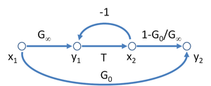
Figure 1 shows a block diagram that leads to the asymptotic gain expression. The asymptotic gain relation also can be expressed as a signal flow graph. See Figure 2. The asymptotic gain model is a special case of the extra element theorem
.

while the direct transmission term G0 is the gain of the system when the return ratio is zero:
These steps can be implemented directly in SPICE
using the small-signal circuit of hand analysis. In this approach the dependent sources of the devices are readily accessed. In contrast, for experimental measurements using real devices or SPICE simulations using numerically generated device models with inaccessible dependent sources, evaluating the return ratio requires special methods.
while in classical feedback theory, in terms of the open loop gain A, the gain with feedback (closed loop gain) is:
Comparison of the two expressions indicates the feedback factor βFB is:
while the open-loop gain is:
If the accuracy is adequate (usually it is), these formulas suggest an alternative evaluation of T: evaluate the open-loop gain and G∞ and use these expressions to find T. Often these two evaluations are easier than evaluation of T directly.
feedback amplifier in Figure 3. The aim is to find the low-frequency, open-circuit, transresistance gain of this circuit G = vout / i in using the asymptotic gain model.
The small-signal equivalent circuit is shown in Figure 4, where the transistor is replaced by its hybrid-pi model
.
.
The return ratio
is found using Figure 5. In Figure 5, the input current source is set to zero, By cutting the dependent source out of the output side of the circuit, and short-circuiting its terminals, the output side of the circuit is isolated from the input and the feedback loop is broken. A test current it replaces the dependent source. Then the return current generated in the dependent source by the test current is found. The return ratio is then T = −ir / it. Using this method, and noticing that RD is in parallel with rO, T is determined as:
where the approximation is accurate in the common case where rO >> RD. With this relationship it is clear that the limits T → 0, or ∞ are realized if we let transconductance
gm → 0, or ∞.
Alternatively G∞ is the gain found by replacing the transistor by an ideal amplifier with infinite gain - a nullor
.
 we simply let gm → 0 and compute the resulting gain. The currents through Rf and the parallel combination of RD || rO must therefore be the same and equal to iin. The output voltage is therefore iin (RD || rO).
Hence
where the approximation is accurate in the common case where rO >> RD.

Examining this equation, it appears to be advantageous to make RD large in order make the overall gain approach the asymptotic gain, which makes the gain insensitive to amplifier parameters (gm and RD). In addition, a large first term reduces the importance of the direct feedthrough factor, which degrades the amplifier. One way to increase RD is to replace this resistor by an active load
, for example, a current mirror
.
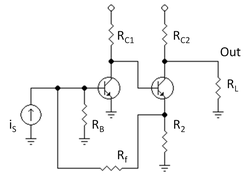
Figure 6 indicates the output node, but does not indicate the choice of output variable. In what follows, the output variable is selected as the short-circuit current of the amplifier, that is, the collector current of the output transistor. Other choices for output are discussed later.
To implement the asymptotic gain model, the dependent source associated with either transistor can be used. Here the first transistor is chosen.
and Kirchhoff's laws
. Resistor R1 = RB // rπ1 and R3 = RC2 // RL. KVL from the ground of R1 to the ground of R2 provides:

KVL provides the collector voltage at the top of RC as

Finally, KCL at this collector provides
Substituting the first equation into the second and the second into the third, the return ratio is found as
Using Ohm's law
, the voltage at the top of R1 is found as
or, rearranging terms,
Using KCL at the top of R2:
Emitter voltage vE already is known in terms of iB from the diagram of Figure 7. Substituting the second equation in the first, iB is determined in terms of iS alone, and G0 becomes:
where
is the return ratioReturn ratio
The return ratio of a dependent source in a linear electrical circuit is the negative of the ratio of the current returned to the site of the dependent source to the current of a replacement independent source...
with the input source disabled (equal to the negative of the loop gain
Loop gain
Loop gain is an engineering term used to quantify the gain of a system controlled by feedback loops. As such, the concept of loop gain is useful in a variety of disciplines. Traditionally, most of those have been in the field of electronics, telecommunications, or control systems...
in the case of a single-loop system composed of unilateral blocks), G∞ is the asymptotic gain and
is the direct transmission term. This form for the gain can provide intuitive insight into the circuit and often is easier to derive than a direct attack on the gain.Figure 1 shows a block diagram that leads to the asymptotic gain expression. The asymptotic gain relation also can be expressed as a signal flow graph. See Figure 2. The asymptotic gain model is a special case of the extra element theorem
Extra element theorem
The Extra Element Theorem is an analytic technique developed by R.D. Middlebrook for simplifying the process of deriving driving point and transfer functions for linear electronic circuits...
.
Definition of terms
As follows directly from limiting cases of the gain expression, the asymptotic gain G∞ is simply the gain of the system when the return ratio approaches infinity:while the direct transmission term G0 is the gain of the system when the return ratio is zero:
Advantages
- This model is useful because it completely characterizes feedback amplifiers, including loading effects and the bilateral properties of amplifiers and feedback networks.
- Often feedback amplifiers are designed such that the return ratio
 is much greater than unity. In this case, and assuming the direct transmission term
  is small (as it often is), the gain
  of the system is approximately equal to the asymptotic gain G∞.
 - The asymptotic gain is (usually) only a function of passive elements in a circuit, and can often be found by inspection.
- The feedback topology (series-series, series-shunt, etc.) need not be identified beforehand as the analysis is the same in all cases.
Implementation
Direct application of the model involves these steps:- Select a dependent source in the circuit.
- Find the return ratioReturn ratioThe return ratio of a dependent source in a linear electrical circuit is the negative of the ratio of the current returned to the site of the dependent source to the current of a replacement independent source...
for that source. - Find the gain G∞ directly from the circuit by replacing the circuit with one corresponding to T = ∞.
- Find the gain G0 directly from the circuit by replacing the circuit with one corresponding to T = 0.
- Substitute the values for T, G∞ and G0 into the asymptotic gain formula.
These steps can be implemented directly in SPICE
SPICE
SPICE is a general-purpose, open source analog electronic circuit simulator.It is a powerful program that is used in integrated circuit and board-level design to check the integrity of circuit designs and to predict circuit behavior.- Introduction :Unlike board-level designs composed of discrete...
using the small-signal circuit of hand analysis. In this approach the dependent sources of the devices are readily accessed. In contrast, for experimental measurements using real devices or SPICE simulations using numerically generated device models with inaccessible dependent sources, evaluating the return ratio requires special methods.
Connection with classical feedback theory
Classical feedback theory neglects feedforward (G0). If feedforward is dropped, the gain from the asymptotic gain model becomes
while in classical feedback theory, in terms of the open loop gain A, the gain with feedback (closed loop gain) is:
Comparison of the two expressions indicates the feedback factor βFB is:
while the open-loop gain is:

If the accuracy is adequate (usually it is), these formulas suggest an alternative evaluation of T: evaluate the open-loop gain and G∞ and use these expressions to find T. Often these two evaluations are easier than evaluation of T directly.
Examples
The steps in deriving the gain using the asymptotic gain formula are outlined below for two negative feedback amplifiers. The single transistor example shows how the method works in principle for a transconductance amplifier, while the second two-transistor example shows the approach to more complex cases using a current amplifier.Single-stage transistor amplifier
Consider the simple FETFet
Fet is a municipality in Akershus county, Norway. It is part of the Romerike traditional region. The administrative centre of the municipality is the village of Fetsund.Fet was established as a municipality on 1 January 1838...
feedback amplifier in Figure 3. The aim is to find the low-frequency, open-circuit, transresistance gain of this circuit G = vout / i in using the asymptotic gain model.
The small-signal equivalent circuit is shown in Figure 4, where the transistor is replaced by its hybrid-pi model
Hybrid-pi model
The hybrid-pi model is a popular circuit model used for analyzing the small signal behavior of bipolar junction and field effect transistors. The model can be quite accurate for low-frequency circuits and can easily be adapted for higher frequency circuits with the addition of appropriate...
.
Return ratio
It is most straightforward to begin by finding the return ratio T, because G0 and G∞ are defined as limiting forms of the gain as T tends to either zero or infinity. To take these limits, it is necessary to know what parameters T depends upon. There is only one dependent source in this circuit, so as a starting point the return ratio related to this source is determined as outlined in the article on return ratioReturn ratio
The return ratio of a dependent source in a linear electrical circuit is the negative of the ratio of the current returned to the site of the dependent source to the current of a replacement independent source...
.
The return ratio
Return ratio
The return ratio of a dependent source in a linear electrical circuit is the negative of the ratio of the current returned to the site of the dependent source to the current of a replacement independent source...
is found using Figure 5. In Figure 5, the input current source is set to zero, By cutting the dependent source out of the output side of the circuit, and short-circuiting its terminals, the output side of the circuit is isolated from the input and the feedback loop is broken. A test current it replaces the dependent source. Then the return current generated in the dependent source by the test current is found. The return ratio is then T = −ir / it. Using this method, and noticing that RD is in parallel with rO, T is determined as:
where the approximation is accurate in the common case where rO >> RD. With this relationship it is clear that the limits T → 0, or ∞ are realized if we let transconductance
Transconductance
Transconductance, also known as mutual conductance, is a property of certain electronic components. Conductance is the reciprocal of resistance; transconductance, meanwhile, is the ratio of the current change at the output port to the voltage change at the input port. It is written as gm...
gm → 0, or ∞.
Asymptotic gain
Finding the asymptotic gain G∞ provides insight, and usually can be done by inspection. To find G∞ we let gm → ∞ and find the resulting gain. The drain current, iD = gm vGS, must be finite. Hence, as gm approaches infinity, vGS also must approach zero. As the source is grounded, vGS = 0 implies vG = 0 as well. With vG = 0 and the fact that all the input current flows through Rf (as the FET has an infinite input impedance), the output voltage is simply −iin Rf. HenceAlternatively G∞ is the gain found by replacing the transistor by an ideal amplifier with infinite gain - a nullor
Nullor
A nullor is a theoretical two-port network composed of a nullator at its input and a norator at its output. Nullors represent an ideal amplifier, having infinite current, voltage, transconductance and transimpedance gain...
.
Direct feedthrough
To find the direct feedthrough we simply let gm → 0 and compute the resulting gain. The currents through Rf and the parallel combination of RD || rO must therefore be the same and equal to iin. The output voltage is therefore iin (RD || rO).Hence
where the approximation is accurate in the common case where rO >> RD.
Overall gain
The overall transresistance gain of this amplifier is therefore:Examining this equation, it appears to be advantageous to make RD large in order make the overall gain approach the asymptotic gain, which makes the gain insensitive to amplifier parameters (gm and RD). In addition, a large first term reduces the importance of the direct feedthrough factor, which degrades the amplifier. One way to increase RD is to replace this resistor by an active load
Active load
An active or dynamic load is a component or a circuit behaving as a current-stable nonlinear resistor. This term may refer to a component of circuit design, or to a type of test equipment.-Circuit design:...
, for example, a current mirror
Current mirror
A current mirror is a circuit designed to copy a current through one active device by controlling the current in another active device of a circuit, keeping the output current constant regardless of loading. The current being 'copied' can be, and sometimes is, a varying signal current...
.
Two-stage transistor amplifier
Figure 6 shows a two-transistor amplifier with a feedback resistor Rf. This amplifier is often referred to as a shunt-series feedback amplifier, and analyzed on the basis that resistor R2 is in series with the output and samples output current, while Rf is in shunt (parallel) with the input and subtracts from the input current. See the article on negative feedback amplifier and references by Meyer or Sedra. That is, the amplifier uses current feedback. It frequently is ambiguous just what type of feedback is involved in an amplifier, and the asymptotic gain approach has the advantage/disadvantage that it works whether or not you understand the circuit.Figure 6 indicates the output node, but does not indicate the choice of output variable. In what follows, the output variable is selected as the short-circuit current of the amplifier, that is, the collector current of the output transistor. Other choices for output are discussed later.
To implement the asymptotic gain model, the dependent source associated with either transistor can be used. Here the first transistor is chosen.
Return ratio
The circuit to determine the return ratio is shown in the top panel of Figure 7. Labels show the currents in the various branches as found using a combination of Ohm's lawOhm's law
Ohm's law states that the current through a conductor between two points is directly proportional to the potential difference across the two points...
and Kirchhoff's laws
Kirchhoff's laws
There are several Kirchhoff's laws, all named after Gustav Robert Kirchhoff:* Kirchhoff's circuit laws* Kirchhoff's law of thermal radiation* Kirchhoff's equations* Kirchhoff's three laws of spectroscopy* Kirchhoff's law of thermochemistry-See also:...
. Resistor R1 = RB // rπ1 and R3 = RC2 // RL. KVL from the ground of R1 to the ground of R2 provides:
KVL provides the collector voltage at the top of RC as
Finally, KCL at this collector provides
Substituting the first equation into the second and the second into the third, the return ratio is found as

Gain G0 with T = 0
The circuit to determine G0 is shown in the center panel of Figure 7. In Figure 7, the output variable is the output current βiB (the short-circuit load current), which leads to the short-circuit current gain of the amplifier, namely βiB / iS:
Using Ohm's law
Ohm's law
Ohm's law states that the current through a conductor between two points is directly proportional to the potential difference across the two points...
, the voltage at the top of R1 is found as

or, rearranging terms,
Using KCL at the top of R2:

Emitter voltage vE already is known in terms of iB from the diagram of Figure 7. Substituting the second equation in the first, iB is determined in terms of iS alone, and G0 becomes:
-

Gain G0 represents feedforward through the feedback network, and commonly is negligible.
Gain G∞ with T → ∞
The circuit to determine G∞ is shown in the bottom panel of Figure 7. The introduction of the ideal op amp (a nullorNullorA nullor is a theoretical two-port network composed of a nullator at its input and a norator at its output. Nullors represent an ideal amplifier, having infinite current, voltage, transconductance and transimpedance gain...
) in this circuit is explained as follows. When T → ∞, the gain of the amplifier goes to infinity as well, and in such a case the differential voltage driving the amplifier (the voltage across the input transistor rπ1) is driven to zero and (according to Ohm's law when there is no voltage) it draws no input current. On the other hand the output current and output voltage are whatever the circuit demands. This behavior is like a nullor, so a nullor can be introduced to represent the infinite gain transistor.
The current gain is read directly off the schematic:
Comparison with classical feedback theory
Using the classical model, the feed-forward is neglected and the feedback factor βFB is (assuming transistor β >> 1):
and the open-loop gain A is:
Overall gain
The above expressions can be substituted into the asymptotic gain model equation to find the overall gain G. The resulting gain is the current gain of the amplifier with a short-circuit load.
Gain using alternative output variables
In the amplifier of Figure 6, RL and RC2 are in parallel.
To obtain the transresistance gain, say Aρ, that is, the gain using voltage as output variable, the short-circuit current gain G is multiplied by RC2 // RL in accordance with Ohm's lawOhm's lawOhm's law states that the current through a conductor between two points is directly proportional to the potential difference across the two points...
:
The open-circuit voltage gain is found from Aρ by setting RL → ∞.
To obtain the current gain when load current iL in load resistor RL is the output variable, say Ai, the formula for current division is used: iL = iout × RC2 / ( RC2 + RL ) and the short-circuit current gain G is multiplied by this loading factor:
Of course, the short-circuit current gain is recovered by setting RL = 0 Ω.
See also
- Return ratioReturn ratioThe return ratio of a dependent source in a linear electrical circuit is the negative of the ratio of the current returned to the site of the dependent source to the current of a replacement independent source...
- Signal-flow graphSignal-flow graphA signal-flow graph is a special type of block diagram—and directed graph—consisting of nodes and branches. Its nodes are the variables of a set of linear algebraic relations. An SFG can only represent multiplications and additions. Multiplications are represented by the weights of the branches;...
- Feedback amplifiers
External links
-